Boosting one tree
at a time
Ferran Muiños
updated: Monday 20210301

Aim of the talk
"Demystify tree ensemble methods and in particular boosted trees"
-
Quick overview of regression
-
Gentle intro to decision trees and tree ensembles
-
What does boosting intend?
-
Some examples along the way
Why ensemble methods in the end of the day?
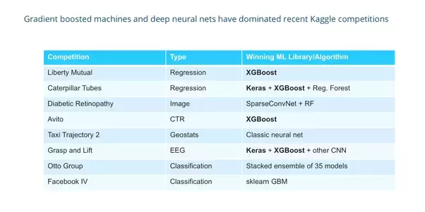
https://www.quora.com/What-machine-learning-approaches-have-won-most-Kaggle-competitions
Regression
X \stackrel{\textrm{dependence}}{\longrightarrow} Y
covariates
response


Regression
X \stackrel{\textrm{dependence}}{\longrightarrow} Y
covariates
response
Problem statement:
Find a function that gives a precise description of the dependence relationship between and :
f
X
Y
Y = f(X) + \varepsilon
Regression
Alternative problem statement:
Given a collection of samples
find a function that provides:
- Low-error approximations (good fit)
- Expected good fit for any dataset of the same kind.
s_1 = \{x_1, y_1\}
\vdots
s_K = \{x_K, y_K\}
f
f(x_i) \sim y_i
X \stackrel{\textrm{dependence}}{\longrightarrow} Y
covariates
response
First example: cell culture
x
y
First example: cell culture
x
y
What patterns do we see?
First example: cell culture
x
y


First example: cell culture
f(x) = \frac{1}{k}\sum_{i \in \mathcal{N_k(x)}} y_i
Average Smoothing
f(x) = \frac{\sum_{i=1}^N K(x - x_i)y_i}{\sum_{i=1}^N K(x - x_i)}
Nadaraya-Watson

K(x)
: bell-shaped kernel


First example: cell culture
Linear
f(x) = ax + b
f(x) = ax^2 + bx + c
Quadratic
First example: cell culture
Parametric methods:
- assume global shape
- very restricted overall
- maybe inaccurate prediction
- maybe easier to interpret
Smoothers:
- agnostic shape
- shape is locally restricted
- useful for prediction
- more difficult to interpret
f(x) = E(Y | X = x)
Whatever the strategy, we want some
f:\mathbb{R}^n \to \mathbb{R}
that satisfies
f(x) = E(Y | X = x)
Whatever the strategy, we want some
f:\mathbb{R}^n \to \mathbb{R}
that satisfies
Applicable to datasets with n covatiates
f(x) = E(Y | X = x)
Whatever the strategy, we want some
f:\mathbb{R}^n \to \mathbb{R}
that satisfies
This is the key!
How do we know what to expect after all?
Data subsets
Dataset
Training dataset
Test dataset
Fit the model
Test the model


Bagging
Bagging = Bootstrap + Aggregating
- Pick several random subsets of samples:
- Train a model with each subset:
- Create a consensus model:
f_1, \ldots, f_K
\mathcal{S}_1, \ldots, \mathcal{S}_K
f = \mathcal{C}(f_1, \ldots, f_K)
"Averaging" is the typical way to reach consensus
f(x) = \frac{1}{K}\sum_{i=1}^K{f_i(x)}
Bagging does a decent work even with weak components
Me learn good
Tree Ensembles
Trees functions
a.k.a. decision trees:
- Have a root where the input goes
- Leaves contain values
- Inner nodes are if-else statements
- If-else conditions are of the form
x_1 \leq 7
x_2 \leq 9
x = (x_1, x_2)
1
2
4
x_i \leq a
Example
x \leq 15
yes
no
x \leq 10
15
7
yes
no
10

1st split
2nd split
What is the best least-squares fitting stump?

?
- Root splits the data:
- Set leaf values:
S_1 \cup S_2
\omega_1 = \textrm{mean}\{y_j\;|\; j\in S_1\}
\omega_2 = \textrm{mean}\{y_j\;|\; j\in S_2\}
?
Which split gives minimum loss?
e.g. loss = RSS
\omega_1
\omega_2
What is the best least-squares fitting tree?
?
- Root splits the data:
- Set leaf values:
S_1 \cup S_2
For which split do we get minimum RSS?

\omega_1 = \textrm{mean}\{y_j\;|\; j\in S_1\}
\omega_2 = \textrm{mean}\{y_j\;|\; j\in S_2\}
\omega_1
\omega_2
Bagging with stumps...


Random Forests

from sklearn.ensemble import RandomForestRegressor

model = RandomForestRegressor(n_estimators=3, max_depth=1)
res = model.fit(temp, rate)
Random Forests
n_estimators=1000,
max_depth=1


n_estimators=1000,
max_depth=2
Gradient Boosting
- Ensemble model
- General framework where weak learners can take any form
- Taking trees as weak learners gives a greedy version of Random Forest
- Derivative of the loss function plays a prominent role --whence the "gradient".
How it works (XGBoost)
- Training Samples:
- Set a loss function e.g.
Instead of fitting a global model to the loss function, training is done by adding one tree at a time (additive training):
- Initialize the model with the constant tree
- Sequential growth. At each step add a new tree
T_0 = 0
s_1 = \{{\bf x}_1, y_1\}
\vdots
s_K = \{{\bf x}_K, y_K\}
L(y,\hat y)
t_m
T_m \leftarrow T_{m-1} + t_m
(y - \hat{y})^2
How it works
Goal: find that minimizes the loss
t_m
T_m \leftarrow T_{m-1} + t_m
\textrm{Loss}_m (\textbf{x}, y) = \sum_{i=1}^K L(y_i, T_{m-1}({\bf x}_i) + t_m({\bf x}_i)) + \Omega(t_m)
The regularization term penalizes the tree complexity.
For example, in XGBoost:
\Omega(t) = \gamma \ell + \frac{1}{2}\lambda \sum_{j=1}^\ell \omega_j^2
is the number of leaves
are the values (or weights) at the leaves
\omega_i
\ell
\Omega
?
\omega_1
\omega_2
How it works
We can provide a second order
Taylor approximation of the Loss function.
- Recall:
- Define:
t_m
\textrm{Loss}_m(\textbf{x}, y) = \sum_{i=1}^K L(y_i, T_{m-1}({\bf x}_i)) + g_it_m({\bf x}_i) + \frac{1}{2}h_it_m({\bf x}_i)^2 + \Omega(t_m)
How do we find ?
f(x +\Delta x) \approx f(x) + f'(x) \Delta x + \frac{1}{2} f''(x) \Delta x^2
g_i = \frac{\partial L}{\partial y} (y_i, T_{m-1}({\bf x_i}))
h_i = \frac{\partial^2 L}{\partial y^2} (y_i, T_{m-1}({\bf x_i}))
?
\omega_1
\omega_2
How it works
t_m
How do we find ?
New goal: minimize this new loss function
\sum_{i=1}^K g_it({\bf x}_i) + \frac{1}{2}h_it({\bf x}_i)^2 + \Omega(t)
Regrouping by leaf, we can write it as a sum of quadratic functions, one for each leaf:
\sum_{i=1}^K [g_i\omega_{\ell({\bf x}_i)} + \frac{1}{2}h_i\omega_{\ell({\bf x}_i)}^2] + \gamma \ell + \frac{1}{2}\lambda\sum_{j=1}^\ell \omega_j^2 =
= \sum_{j=1}^\ell [(\sum_{i\in I_j} g_i)\omega_j + \frac{1}{2}(\lambda + \sum_{i\in I_j} h_i)\omega_j^2] + \gamma \ell
?
\omega_1
\omega_2
How it works
t_m
How do we find ?
If the tree structure of t is fixed, then the optimal weights for each leaf are given by:
G_j = \sum_{i\in I_j} g_i
\omega_j^* = - \frac{G_j}{H_j + \lambda}
H_j = \sum_{i\in I_j} h_i
where and
Evaluating the new loss on gives a scoring on each possible tree structure.
Trees are grown greedily so that this scoring keeps decreasing at every step.
\omega_j^* = - \frac{G_j}{H_j + \lambda}
?
\omega_1
\omega_2
How it works
Example of a tree structure:
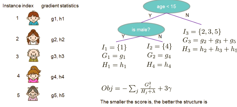
How it works
Now that we have a way to measure how good a tree is, ideally we would enumerate all possible trees and pick the best one. In practice, however, this is intractable.
?
\omega_1
\omega_2
?
\omega_1
\omega_2
?
\omega_2
\omega_3
Is the new split beneficial or not?
Optimal tree structure is searched for iteratively
Tunning hyperparams
- loss function
- learning rate a.k.a. shrinkage:
- number of estimators (trees)
- maximum depth of trees
- randomization rules:
- subset of samples (bagging, out-of-bag error)
- per-tree/per-split subset of covariates
- regularization parameters
We can introduce rules to constraint the search for each update. These rules define the "learning style" of the model.
T \leftarrow T_{m-1} + \nu \cdot t_m
\nu
Why Tree Ensembles?
Upsides:
- Non-parametric (shape agnostic)
- Up to a variety of regression and classification tasks
- Modelling flexibility
- Admit a large number of covariates
- Good prediction accuracy
- Good at capturing interactions between covariates by design
- Interpretation is feasible: ranking variables, partial dependence
- Efficient functions
Downsides:
- Steeper learning curve for users
Why gradient boosting?
Upsides:
- Same reasons why I like Random Forests, plus...
- Very good accuracy with fewer learners (greedy).
- Excellent XGBoost implementation (R, Python).
- Many model design options at reach.
Downsides:
- Sequential by design, hence intrinsically slower to train than other methods like RF.
- Hyperparameter tuning.
References
-
Freund Y, Schapire R A short introduction to boosting
-
Hastie T, Tibshirani R, Friedman J The Elements of Statistical Learning
-
Natekin A, Knoll A Gradient boosting machines, a tutorial
-
XGBoost Documentation: https://xgboost.readthedocs.io/en/latest
Gradient boosting seminar at Bioinfo UPF
By Ferran Muiños
Gradient boosting seminar at Bioinfo UPF
A gentle introduction to ensemble tree models and gradient boosting for regression.


