Gradient Boosting
one tree at a time

Aim of the talk
"Demystify tree ensemble methods"
-
Quick overview of regression
-
Gentle intro to decision trees and tree ensembles
-
What does gradient boosting intend?
-
Practical usage
-
Some examples along the way
Regression
X \stackrel{\textrm{dependence}}{\longrightarrow} Y
covariates
response


Regression
X \stackrel{\textrm{dependence}}{\longrightarrow} Y
covariates
response
Problem statement:
Find a function that gives a precise description of the dependence relationship between and :
f
X
Y
Y = f(X) + \varepsilon
Regression
Alternative problem statement:
Given a collection of samples
find a function that provides:
- Low-error approximations (good fit)
- Expected good fit for any dataset of the same kind.
s_1 = \{x_1, y_1\}
\vdots
s_K = \{x_K, y_K\}
f
f(x_i) \sim y_i
X \stackrel{\textrm{dependence}}{\longrightarrow} Y
covariates
response
First example: cell culture
x
y
First example: cell culture
x
y
What patterns do we see?
First example: cell culture
x
y

Perfect fit!
But do not expect it to fit new data :(

First example: cell culture
f(x) = \frac{1}{k}\sum_{i \in \mathcal{N_k(x)}} y_i
Average Smoothing
f(x) = \frac{\sum_{i=1}^N K(x - x_i)y_i}{\sum_{i=1}^N K(x - x_i)}
Nadaraya-Watson

K(x)
: bell-shaped kernel


First example: cell culture
Linear
f(x) = ax + b
f(x) = ax^2 + bx + c
Quadratic
First example: cell culture
Parametric methods:
- assume global shape
- very restricted overall
- maybe inaccurate prediction
- maybe easier to interpret
Smoothers:
- agnostic shape
- shape is locally restricted
- useful for prediction
- more difficult to interpret
f(x) = E(Y | X = x)
Whatever the strategy, we want some
f:\mathbb{R}^n \to \mathbb{R}
that satisfies
f(x) = E(Y | X = x)
Whatever the strategy, we want some
f:\mathbb{R}^n \to \mathbb{R}
that satisfies
Applicable to datasets with n covatiates
f(x) = E(Y | X = x)
Whatever the strategy, we want some
f:\mathbb{R}^n \to \mathbb{R}
that satisfies
This is the key!
How do we know what to expect after all?
Data subsets
Dataset
Training dataset
Test dataset
Fit the model
Test the model


Bagging
Bagging = Bootstrap + Aggregating
- Pick several random subsets of samples:
- Train a model with each subset:
- Create a consensus model:
f_1, \ldots, f_K
\mathcal{S}_1, \ldots, \mathcal{S}_K
f = \mathcal{C}(f_1, \ldots, f_K)
"Averaging" is the typical way to reach consensus
f(x) = \frac{1}{K}\sum_{i=1}^K{f_i(x)}
Bagging does a decent work even with weak models...
I am a small tree.
Learn weak, die hard.
Tree Ensembles
Trees (a.k.a. decision trees) are functions of a particular kind:
- Have a root where the input goes
- Leaves are values
- Inner nodes are if-else statements
- If-else conditions are of the form
x_1 \leq 7
x_2 \leq 9
x = (x_1, \ldots, x_n)
1
2
4
x_i \leq a
Example
x \leq 15
yes
no
x \leq 10
15
7
yes
no
10

1st split
2nd split
What is the best least-squares fitting tree?

?
- Root splits the data:
- Set leaf values:
S_1 \cup S_2
\mu_1 = \textrm{mean}\{y_j\;|\; j\in S_1\}
\mu_2 = \textrm{mean}\{y_j\;|\; j\in S_2\}
?
For which split do we get minimum RSS?
What is the best least-squares fitting tree?
?
- Root splits the data:
- Set leaf values:
S_1 \cup S_2
\mu_1 = \textrm{mean}\{y_j\;|\; j\in S_1\}
\mu_2 = \textrm{mean}\{y_j\;|\; j\in S_2\}
YES!
For which split do we get minimum RSS?

Bagging with stumps...


Random Forests

from sklearn.ensemble import RandomForestRegressor

model = RandomForestRegressor(n_estimators=3, max_depth=1)
res = model.fit(temp, rate)
Random Forests
n_estimators=1000,
max_depth=1


n_estimators=1000,
max_depth=2
Gradient Boosting
Greedy cousin of the Random Forest:
- Model = sum of trees
- Trees are computed sequentially
+
+ \;\ldots
How it works
Fix a loss function: e.g.
Initialize the model with an educated guess:
At each step we find a new tree :
The tree is such that the following "loss" is small:
T_0
Training Samples:
s_1 = \{x_1, y_1\}
\vdots
s_K = \{x_K, y_K\}
L(y, \hat{y})
t_m
T \leftarrow T_{m-1} + \nu \cdot t_m
\frac{1}{2}\sum_{i=1}(y_i - \hat{y}_i)^2
t_m
\textrm{Loss}_m (\textbf{x}) = \sum_{i=1}^K L(y_i, T_{m-1}(x_i) + t_m(x_i)) + \Omega(t_m)
m
How it works
Using Taylor's expansion this can be re-written:
The tree is such that the following objective is minimized:
t_m
\textrm{Obj}_m = \sum_{i=1}^K L(y_i, T_{m-1}(x_i)) + g_it_m(x_i) + h_it_m(x_i)^2 + \Omega(t_m)
\sum_{i=1}^K g_it_m(x_i) + h_it_m(x_i)^2 + \Omega(t_m)
How it works
The tree is such that the following objective is minimized:
t_m
\sum_{i=1}^K g_it_m(x_i) + h_it_m(x_i)^2 + \Omega(t_m)
These pseudo-residuals are computed using the first derivative of the loss function L
These factors are computed using the second-derivative of the loss function L
Regularization term
Tunning hyperparams
- loss function
- learning rate a.k.a. shrinkage:
- number of estimators (trees)
- maximum depth of trees
- randomization rules:
- subset of samples (size)
- per-tree/per-split subset of covariates (ratio)
- regularization parameters
We can introduce rules to constraint the search for each update. These rules define the "learning style" of the model.
T \leftarrow T_{m-1} + \nu \cdot t_m
\nu
Why Tree Ensembles?
Upsides:
- Non-parametric (shape agnostic)
- Up to a variety of regression and classification tasks
- Modelling flexibility
- Admit a large number of covariates
- Good prediction accuracy
- Good at capturing interactions between covariates by design
- Interpretation is feasible: ranking variables, partial dependence
- Efficient functions
Downsides:
- Steeper learning curve for users
Why gradient boosting?
Upsides:
- Same reasons why I like Random Forests, plus...
- Very good accuracy with fewer learners (greedy).
- Excellent XGBoost implementation (R, Python).
- Many model design options at reach.
Downsides:
- Sequential by design, hence intrinsically slower to train than other methods like RF.
- Hyperparameter tuning.
Hands-on

GB hands-on
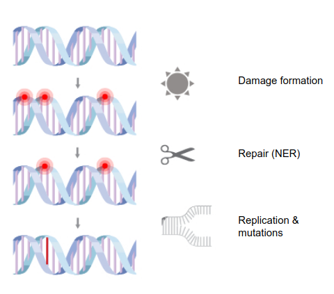
Dataset: UV-induced CPD (cyclobutane pyrimidine dimer) in human skin fibroblasts
Samples: 1Mb chunks
Response: CPD counts per chunk
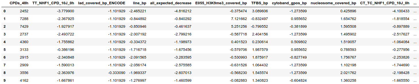
Covariates: Annotated coverage by chromatin-associated structures and enrichment of histone modifications enrichment.
GB hands-on
Challenges
Many covariates: from 20 to 1000+
Many interactions expected
Want accurate prediction without killing interpretation
Parameters
params = {

'objective': 'reg:linear',
'n_estimators':        15000,
'subsample':          0.5,
'colsample_bytree':          0.5,
'learning_rate':        0.001,
'max_depth':            4,

...

}
Accuracy and CV


0.5 Fold
Accuracy

Partial model with single covariate (~ 0.3 Var Explained)
Full Model (~ 0.9 Var Explained)
Feature Importance
Several choices in most frameworks
- Number of splits each covariate contributes.
- Gain: mean decrease of error every time a covariate is used in a split.
- Permutation: how the error increases after "noising" a covariate.
-
Attribution: model the effect of each covariate in each sample.
Feature Importance
- Number of splits each covariate contributes.
- Gain: mean decrease of error every time a covariate is used in a split.
- Permutation: how the error increases after "noising" a covariate.
-
Attribution models: model the effect of each covariate in each sample.
We use an attribution model based on
Shapley values (cooperative game theory)
"average effect of adding a feature to predict a given sample"
Feature Importance


Partial Dependence & Interaction


Example with H3K27ac
Kudos to...
-
Valiant (1984): PAC learning models
-
Kearns and Valiant (1988): first to pose the question of whether a “weak” learning algorithm which performs just slightly better than random guessing [PAC] can be “boosted” into an arbitrarily accurate “strong” learning algorithm.
-
Schapire (1989): first provable polynomial-time boosting algorithm.
-
Freund (2000): improved efficiency and caveats.
-
Many others...
Kudos to...

References
-
Distributed Machine Learning Common Codebase https://xgboost.readthedocs.io/en/latest/model.html
-
Freund Y, Schapire R A short introduction to boosting
-
Hastie T, Tibshirani R, Friedman J The Elements of Statistical Learning
-
Lundberg S, Lee S-I Consistent individualized feature attribution for tree ensembles
-
Natekin A, Knoll A Gradient boosting machines, a tutorial
Gradient boosting seminar at IRB
By Ferran Muiños
Gradient boosting seminar at IRB
A gentle introduction to ensemble tree models and gradient boosting for regression. Presented at the BBG-SBNB joint seminar at IRB Barcelona.


