Simulation of nanostructures
László Oroszlány
KRFT, ELTE
Trends in Nanotechnology @ BME
DFT
- Basics
- Functionals
- When to use DFT ?
- When not to use DFT ?
- state of the art:
codes and stories
Landauer
- Landauer's approach
- Green's functions
- Transmission
- Generalizations
- state of the art:
codes and stories
Outline
This is meant to be an apetizer...

But it might feel like...

Density Functional Theory
Act I
The many body problem
\displaystyle{\hat{H}=\sum_i \frac{\hat{p_i}^2}{2m} +\sum_{ij} \hat{V}_{ee}(r_i-r_j)+\sum_{ij} \hat{V}_{eN}(r_i-R_j) }
\hat H\psi_n(r_1,r_2,\ldots)=E_n\psi_n(r_1,r_2,\ldots)
Universal
System specific
an AWFULL LOT \(\approx 10^{23}\) of variables..
Hohenberg–Kohn theorems
Theorem 1: The external potential (and hence the total energy), is a unique functional of the electron density.
Theorem 2: The ground state density minimizes the total energy functional.
\exists! E_{Tot}[n(r)]
\displaystyle n(r)=\int \mathrm{d}r_2 \mathrm{d}r_3\ldots|\psi(r,r_2,r_3,\ldots)|^2
\left . \displaystyle \delta E_{Tot}[n(r)] \right |_{n_{GS}(r)}=0
Phys. Rev. 136, B864 (1964)
Recap on Functionals
a function maps numbers to numbers:

\mathbb{R}\rightarrow \mathbb{R}
x\rightarrow x^2-x-2
a functional maps functions to numbers:
(\mathbb{R}\rightarrow\mathbb{R})\Rightarrow\mathbb{R}
(x\rightarrow x^2-x-2)\Rightarrow -\frac{9}{2}
\displaystyle\int_{-1}^2 (x^2-x-2)\mathrm{d}x=-\frac{9}{2}
Kohn–Sham equations and the scf loop
E_{Tot}[n(r)]=T[n]+E_{ext}[n]+E_{H}[n]+E_{xc}[n]
\displaystyle n(r)=\sum_{i=0}^{N_{occ}} |\phi_i(r)|^2
T[n]=\displaystyle\sum_i \left \langle\phi_i\right|-\frac{\hbar^2\Delta}{2m}\left |\phi_i\right\rangle
\displaystyle E_{ext}=\int V_{ext}(r)n(r) \mathrm{d}r
\displaystyle E_{H}=\frac{e^2}{2}\int \frac{n(r')n(r)}{|r-r'|} \mathrm{d}r\mathrm{d}r'
\displaystyle E_{xc}=?=\mathcal{F}[n(r)]
\displaystyle v_{eff}(r)=\frac{\delta}{\delta n}[E_{ext}+E_{H}+E_{xc}]
\displaystyle \left (\frac{-\hbar^2\Delta}{2m}+v_{eff}(r)\right) \phi_i(r)=E_i \phi_i(r)
Phys. Rev. 140, A1133 (1965)
Functionals of exchange and correlation
- S: The Slater exchange, ρ4/3 with theoretical coefficient of 2/3, also referred to as Local Spin Density exchange [Hohenberg64, Kohn65, Slater74]. Keyword if used alone: HFS.
- XA: The XAlpha exchange, ρ4/3 with the empirical coefficient of 0.7, usually employed as a standalone exchange functional, without a correlation functional [Hohenberg64, Kohn65, Slater74]. Keyword if used alone: XAlpha.
- B: Becke’s 1988 functional, which includes the Slater exchange along with corrections involving the gradient of the density [Becke88b]. Keyword if used alone: HFB.
- PW91: The exchange component of Perdew and Wang’s 1991 functional [Perdew91, Perdew92, Perdew93a, Perdew96, Burke98].
- mPW: The Perdew-Wang 1991 exchange functional as modified by Adamo and Barone [Adamo98].
- G96: The 1996 exchange functional of Gill [Gill96, Adamo98a].
- PBE: The 1996 functional of Perdew, Burke and Ernzerhof [Perdew96a, Perdew97].
- O: Handy’s OPTX modification of Becke’s exchange functional [Handy01, Hoe01].
- TPSS: The exchange functional of Tao, Perdew, Staroverov, and Scuseria [Tao03].
- RevTPSS: The revised TPSS exchange functional of Perdew et. al. [Perdew09, Perdew11].
- BRx: The 1989 exchange functional of Becke [Becke89a].
- PKZB: The exchange part of the Perdew, Kurth, Zupan and Blaha functional [Perdew99].
- wPBEh: The exchange part of screened Coulomb potential-based final of Heyd, Scuseria and Ernzerhof (also known as HSE) [Heyd03, Izmaylov06, Henderson09].
- PBEh: 1998 revision of PBE [Ernzerhof98].
- VWN: Vosko, Wilk, and Nusair 1980 correlation functional(III) fitting the RPA solution to the uniform electron gas, often referred to as Local Spin Density (LSD) correlation [Vosko80] (functional III in this article).
- VWN5: Functional V from reference [Vosko80] which fits the Ceperly-Alder solution to the uniform electron gas (this is the functional recommended in [Vosko80]).
- LYP: The correlation functional of Lee, Yang, and Parr, which includes both local and non-local terms [Lee88, Miehlich89].
- PL (Perdew Local): The local (non-gradient corrected) functional of Perdew (1981) [Perdew81].
- P86 (Perdew 86): The gradient corrections of Perdew, along with his 1981 local correlation functional [Perdew86].
- PW91 (Perdew/Wang 91): Perdew and Wang’s 1991 gradient-corrected correlation functional [Perdew91, Perdew92, Perdew93a, Perdew96, Burke98].
- B95 (Becke 95): Becke’s τ-dependent gradient-corrected correlation functional (defined as part of his one parameter hybrid functional [Becke96]).
- PBE: The 1996 gradient-corrected correlation functional of Perdew, Burke and Ernzerhof [Perdew96a, Perdew97].
- TPSS: The τ-dependent gradient-corrected functional of Tao, Perdew, Staroverov, and Scuseria [Tao03].
- RevTPSS: The revised TPSS correlation functional of Perdew et. al. [Perdew09, Perdew11].
- KCIS: The Krieger-Chen-Iafrate-Savin correlation functional [Rey98, Krieger99, Krieger01, Toulouse02].
- BRC: Becke-Roussel correlation functional [Becke89a].
- PKZB: The correlation part of the Perdew, Kurth, Zupan and Blaha functional [Perdew99].
- VP86: VWN5 local and P86 non-local correlation functional.
- V5LYP: VWN5 local and LYP non-local correlation functional.
- VSXC: van Voorhis and Scuseria’s τ-dependent gradient-corrected correlation functional [VanVoorhis98].
- HCTH/*: Handy’s family of functionals including gradient-corrected correlation [Hamprecht98, Boese00, Boese01]. HCTH refers to HCTH/407, HCTH93 to HCTH/93, HCTH147 to HCTH/147, and HCTH407 to HCTH/407. Note that the related HCTH/120 functional is not implemented.
- tHCTH: The τ-dependent member of the HCTH family [Boese02]. See also tHCTHhyb below.
- B97D: Grimme’s functional including dispersion [Grimme06]. B97D3 requests the same but with Grimme’s D3BJ dispersion [Grimme11].
- M06L [Zhao06a], SOGGA11 [Peverati11], M11L [Peverati12], MN12L [Peverati12c] N12 [Peverati12b] and MN15L [Yu16a] request these pure functionals from the Truhlar group.
\displaystyle E^{LDA}_{xc}[n]=\int \epsilon_{LDA}(n)n(r) \mathrm{d}r
\displaystyle E^{GGA}_{xc}[n]=\int \epsilon_{GGA}(n,|\nabla n|)n(r) \mathrm{d}r
\displaystyle E^{LSDA}_{xc}[n_\uparrow,n_\downarrow]=\int \epsilon_{LSDA}(n_\uparrow,n_\downarrow)n(r) \mathrm{d}r


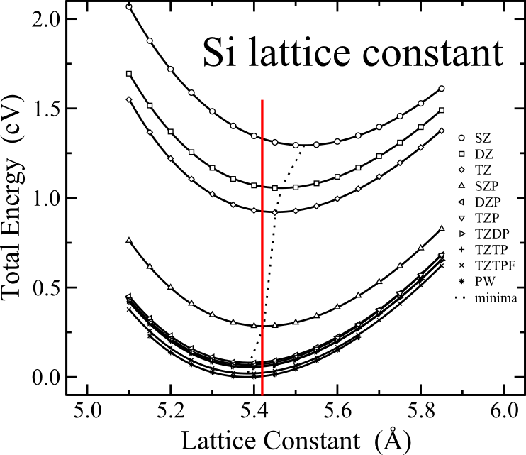
The choice of basis
\displaystyle\phi_i(r)=\sum_pa_{ip}\chi_p(r)
| PRO | CON | |
|---|---|---|
|
Plane waves |
-simple to implement -one convergence parameter |
- resource hungry - big basis set needed |
| Atomic like orbitals | - small basis - sparse matrix methods - scales to BIG systems |
-harder to implement -many things influence convergence |
|
KKR method baseless method.. relies on scattering approach and Green's functons |
-relativistic effects are easy -standard for magnetic systems -most accurate for some problems |
-harder to implement -smaller community -some features not yet implemented.. |
\chi_p(r)=\mathrm{e}^{\mathrm{i}pr}
\chi_{nlm}(r)=R_{nl}(\rho)Y_{l}^m(\hat{r})
Pseudopotentials

Motivation:
- Reduction of basis set size
- Reduction of number of electrons
- Inclusion of relativistic and other effects
Approximations:
- One-electron picture.
- The small-core approximation
What is DFT good at?
- structural properties
- electronic structure of simple systems


Failures of DFT
- GAPs
- Strong(ish) interactions


LDA+U:
J. Phys.: Cond. Matt. 9,767 (1997)
DMFT:
Phys. Rev. Lett. 62, 324 (1989)
QMC:
Rev. Mod. Phys. 73, 33 (2001)
GW:
Phys. Rev. 139, A796 (1965)
BSE:
Phys. Rev. Lett. 75, 818 (1995)
State of the art-VASP

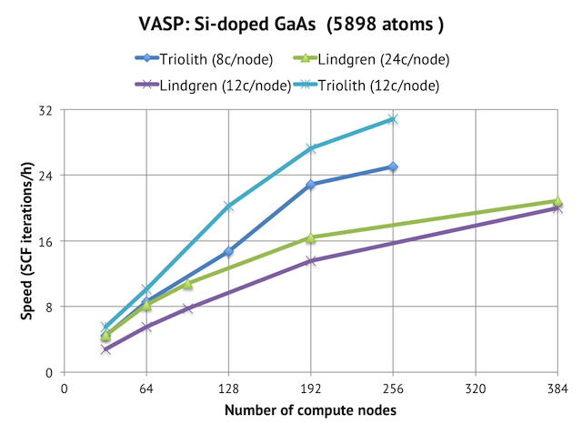
6000 atom
3000 proc
120s/scf
Massively
parallel

Phonon spectrum
J. Chem. Phys. 143, 064710 (2015)
Excitations with
GW method
Phys. Rev. B 75, 235102 (2007)
https://www.vasp.at/
State of the art-Siesta
J. Phys.: Cond. Matt. 27, 054004 (2015)
J. Phys.: Cond. Matt. 26, 305503 (2014)
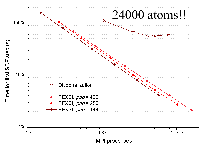
6000 atom
2000 proc
10 sec/scf
SIESTA-PEXSI parallelization
New J. Phys., 16, 093029 (2014)
Phys. Rev. B 65, 165401 (2002)
Local quantities (e.g. STM)
Ideal as an input for transport calculations
https://launchpad.net/siesta
State of the art-KKR


KKRNano @ http://www.judft.de/ massive parallelization
PRB 94, 104511 (2016)
abinitio superconductivity
PRB 89, 224401 (2014)
finite temperature magnetism
PRB 82, 024411 (2010)
ARPES+DMFT
Budapest
München
Jülich
Landauer's Approach
Act II
Conductance quantum
V_L
V_R
\sigma=\frac{e^2}{h}
I
I=\sigma\delta V
\approx 3.874\times 10^{-5} \Omega^{-1}
IBM J. Res. Dev. 1, 223 (1957 )
Conductance of a sample
V_L
V_R
\sigma=\frac{e^2}{h}T
T
IBM J. Res. Dev. 1, 223 (1957 )
Green's functions
\hat{H}_0 =
\begin{pmatrix}
\hat{H}_{s} & 0\\
0 & \hat{H}_{leads}
\end{pmatrix}
\hat{V}=\left(\begin{array}{cc}
0 & \hat{V}_{SL}\\
\hat{V}_{SL}^{\dagger} & 0
\end{array}\right)
\hat{G}_0=(E-\hat{H}_0)^{-1}
\hat{G}=(\hat{G}_0^{-1}-\hat{V})^{-1}
The structure of \( V\) is such that in order to find matrix elements of \(G\) in the neighborhood of the scatterer one only need to invert a FINITE matrix!
Dyson's equation
\hat{H}=\hat{H}_0+\hat{V}
How to get \(T\)?
\hat{G}\text{ from :}
\hat{H}\text{ from :}
- from TB
- fitting to DFT
- directly from DFT
T=\mathrm{Tr}[t^\dagger t]
- take \(\hat{H}\)
- get \(\hat{G}_0\)
- use Dyson's
S_{pq}=\mathrm{i}\sqrt{v_pv_q}\left \langle \phi_p \right |G\left | \phi_q \right \rangle-\delta_{pq}
the scattering matrix:

S=\begin{pmatrix}
r&t'\\
t&r'
\end{pmatrix}
two terminal case:
Fisher-Lee relation: Phys. Rev. B 23, 6851(R) (1981)
Extension to non-equilibrium
Steady state current due to a finite bias.
\displaystyle I=\int_{\mu_R}^{\mu_L}T(E)\mathrm{d}E

Non-equilibrium population of scatterer needs to be taken in to account! \(\Rightarrow\) Keldysh formalism
H. Haug and A. P. Jauho, Quantum Kinetics in Transport and Optics of Semiconductors
Example
Negative differential resistance
in molecular junctions:
Nanotechnology 19, 455203 (2008)
Extension to include Interactions
New Journal of Physics 16 093029 (2014)
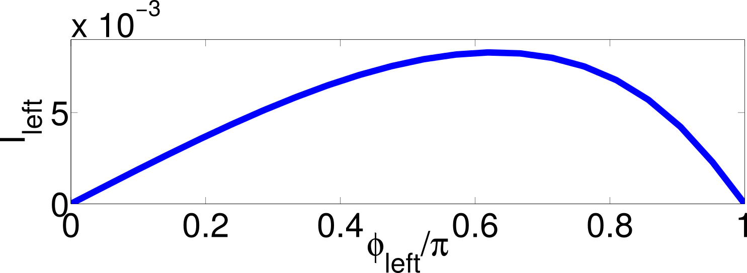
Extension to include Superconductivity

Phys. Rev. B 93, 224510 (2016)
\displaystyle J=\frac{1}{\pi}\mathrm{Im}\int_\Gamma f(z)\mathrm{Tr}[\hat{\mathcal{G}}_{BdG}(z)\hat{J}_{BdG}]
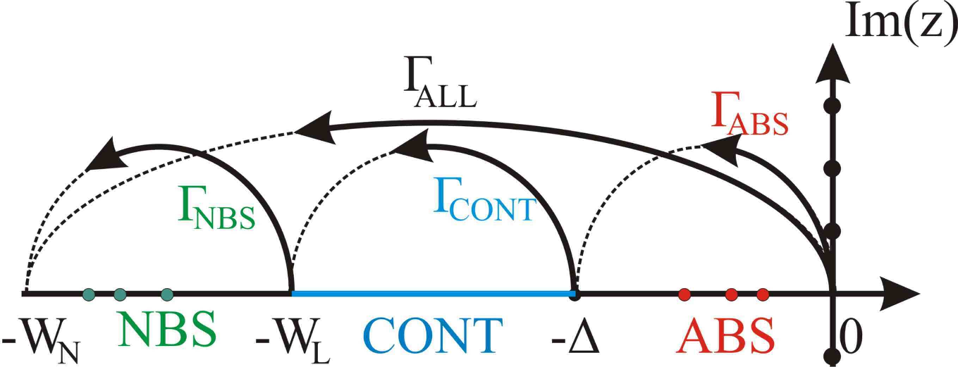
\mathcal{\hat H}_{BdG}=\begin{pmatrix}
\hat{H} & \hat{\Delta} \\
\hat{\Delta}^\dagger & -\hat{H}^*
\end{pmatrix}
https://kwant-project.org/
written in python, ideal for quick and dirty calculations
2x100x400 site disordered topological insulator
quantum Hall effect
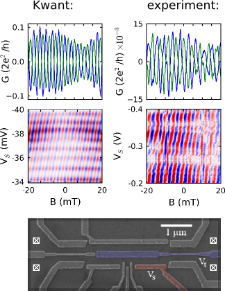
flying qbit
Equus
http://eqt.elte.hu/equus/home
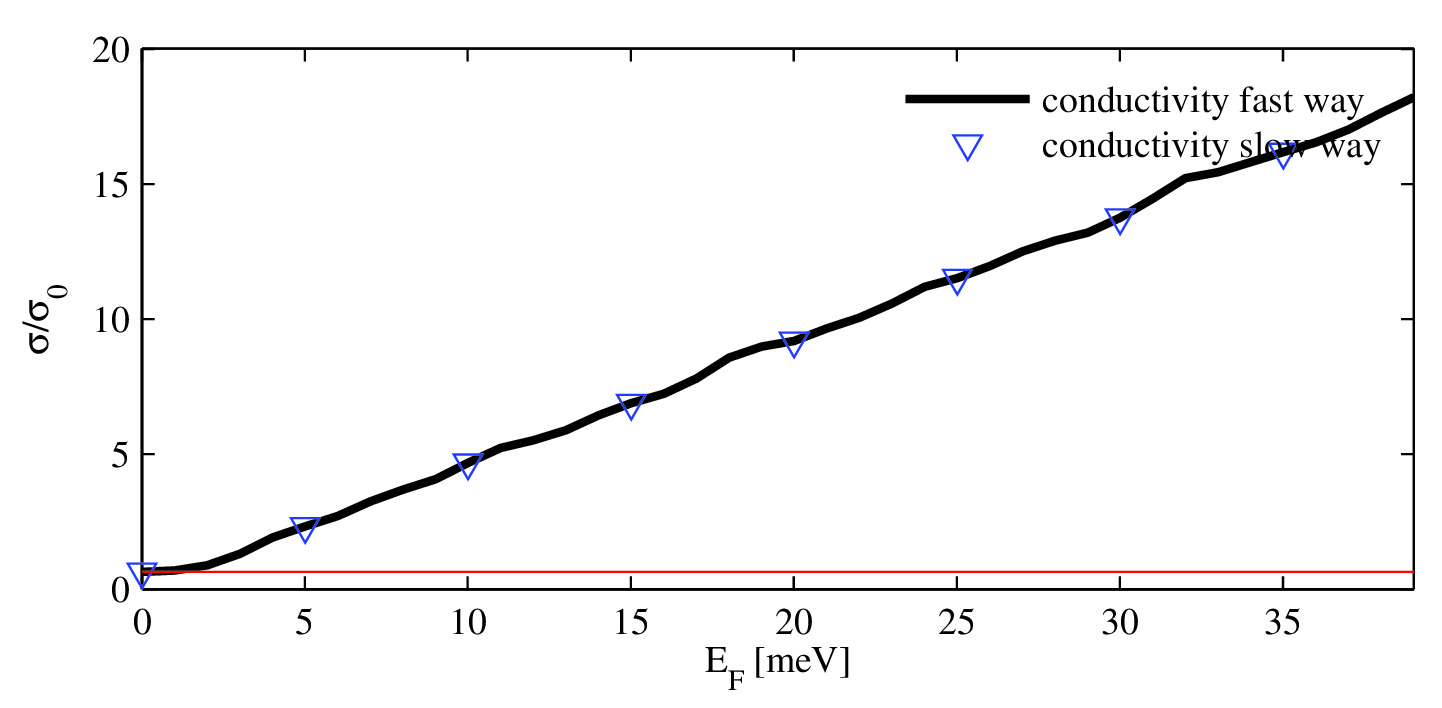
conductivity of a 4\(\mu m\) wide graphene ribbon
graphene ribbon antidot in \(\mathbf{B}\) field
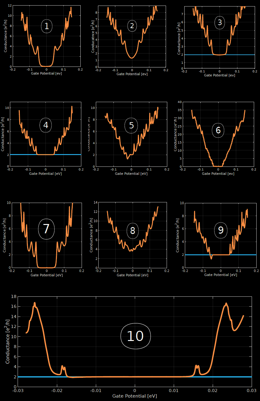
1\(\mu m \times \) 1\(\mu m\)
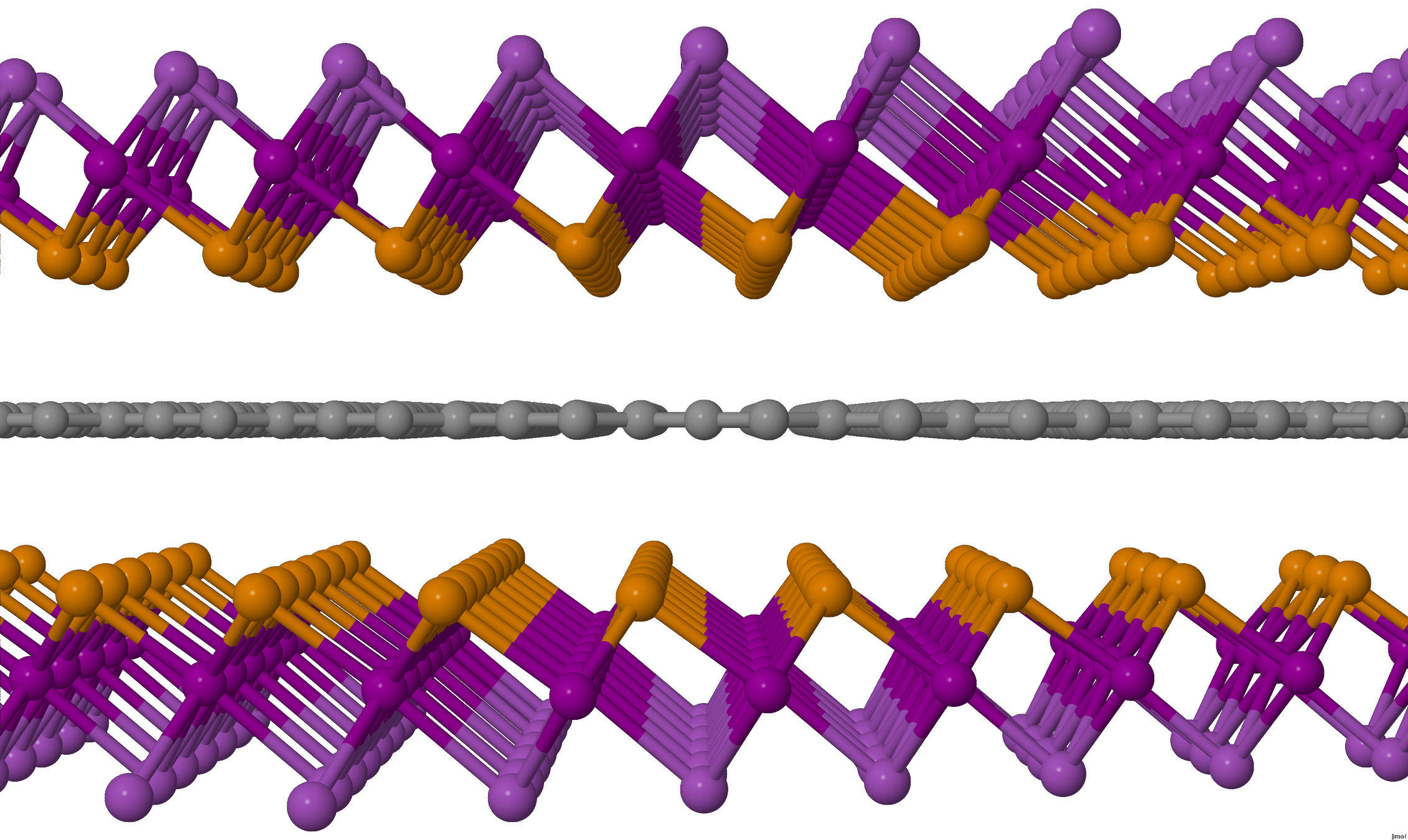
BiTeI/graphene/BiTeI sandwitch

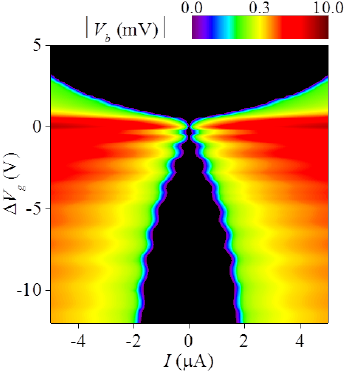
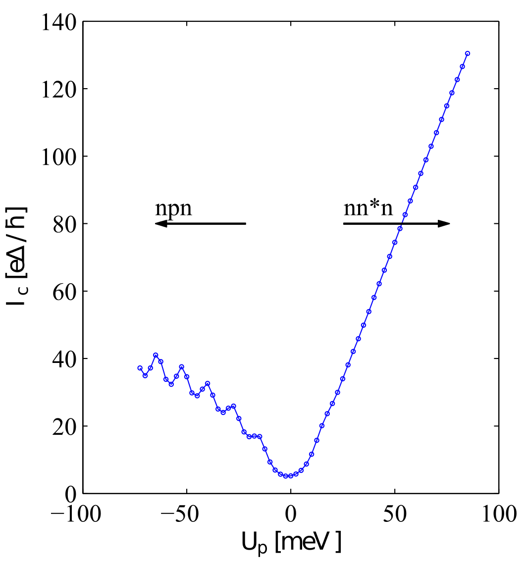
graphene Josephson junction
Gollum
Multi terminal calculations
Statistical analysis of environmental effects
http://www.physics.lancs.ac.uk/gollum/
Magneto transport
thermoelectric properties
A Multi scale story: Indium MCBJ
Makk et al., Phys. Rev. Lett. 107 276801 (2011)
Take home message
- Chemically specific simulation of simple quantities with a cople of thousand atoms!
- Simple quantities of simple models with milions of degrees of freedom!
- Quantites that require an energy integral as a rule of thumb require one order of magnitude more resources!
- Full many body treatment of large scales is still a challenge!

Copy of Trends_in_Nano_at_BME
By Gergő Kukucska


