INTRODUCTION TO QUANTUM MECHANICS
CLASSICAL PHYSICS IS COMPLETE
PV = n R T
H(p,q) = T(p) + V(q)
\begin{cases}
\nabla \cdot \mathbf{E} = \frac{\rho}{\varepsilon_0} \\
\nabla \cdot \mathbf{B} = 0 \\
\nabla \times \mathbf{E} = -\frac{\partial \mathbf{B}}{\partial t} \\
\nabla \times \mathbf{B} = \mu_0 \bigg( \mathbf{J} + \varepsilon_0 \frac{\partial \mathbf{E}}{\partial t} \bigg)
\end{cases}
HAMILTONIAN MECHANICS
MAXWELL'S EQUATIONS
THERMODYNAMICS
A FEW CRACKS STAR SHOWING
THE PHOTOELECTRIC EFFECT
V_c
\pm V_c
A FEW CRACKS STAR SHOWING
THE BLACK BODY SPECTRUM
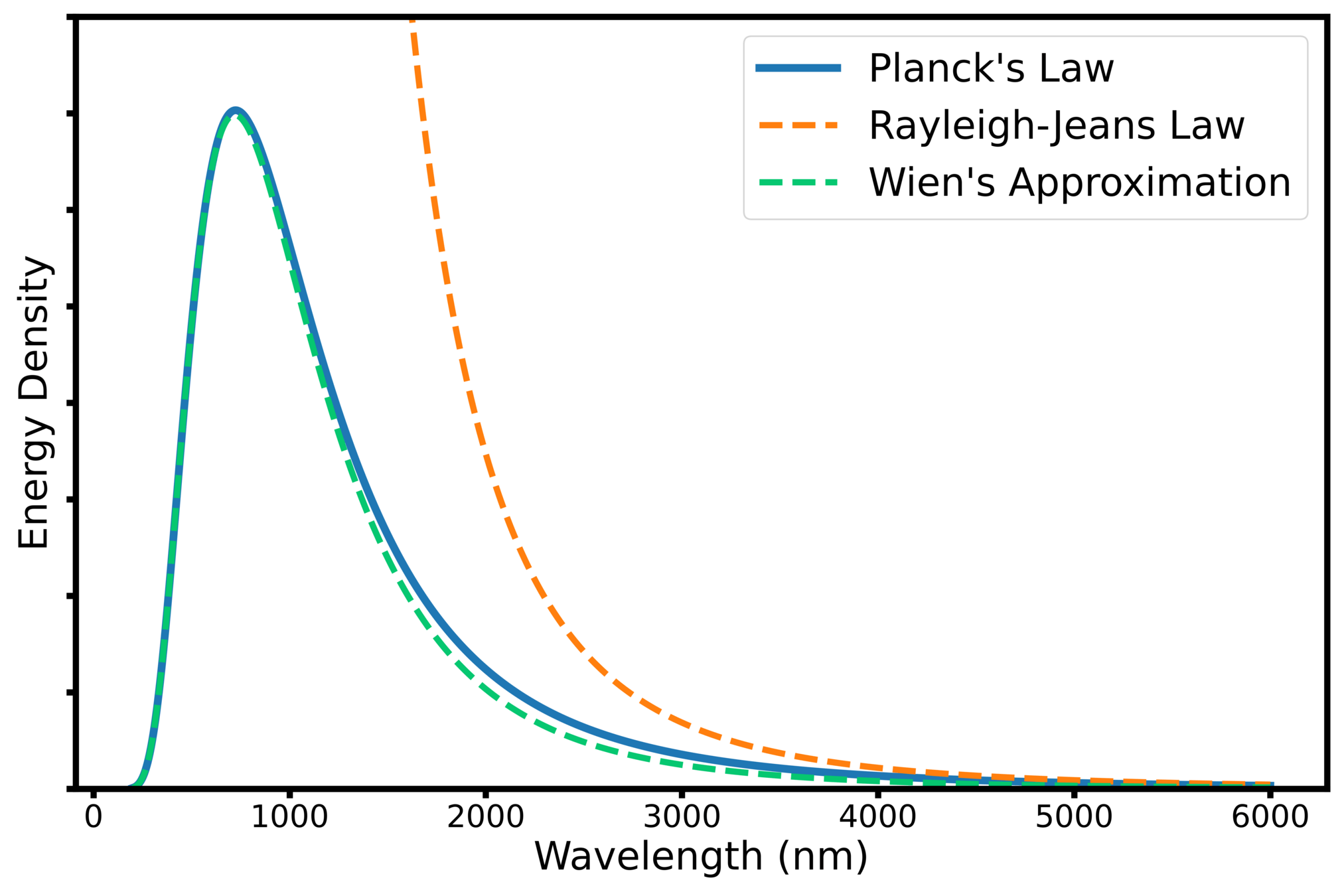
\begin{cases}
u_{\lambda}(\lambda, T) = \frac{8 \pi h c}{\lambda^5} \left( \frac{1}{e^{h c / (\lambda k_BT)} - 1} \right) \\
u_{\nu}(\nu, T) = \frac{8\pi h ν^3}{c^3} \left( \frac{1}{e^{h\nu / (k_B T)} - 1} \right)
\end{cases}
\begin{cases}
u_{\lambda}(\lambda, T) = \frac{8 \pi k_B T}{\lambda^4} \\
u_{\nu}(\nu, T) = \frac{8 \pi ν^2 k_B T}{c^3}
\end{cases}
\begin{cases}
u_{\lambda}(\lambda, T) = 8 \pi h c \frac{e^{ -h c / (\lambda k_B T)})}{\lambda^{5}} \\
u_{\nu}(\nu, T) = \left( \frac{8 \pi h \nu^3}{c^3} \right) e^{ -\frac{h \nu}{k_B T}}
\end{cases}
A FEW CRACKS STAR SHOWING
THE BLACK BODY SPECTRUM
A FEW CRACKS STAR SHOWING
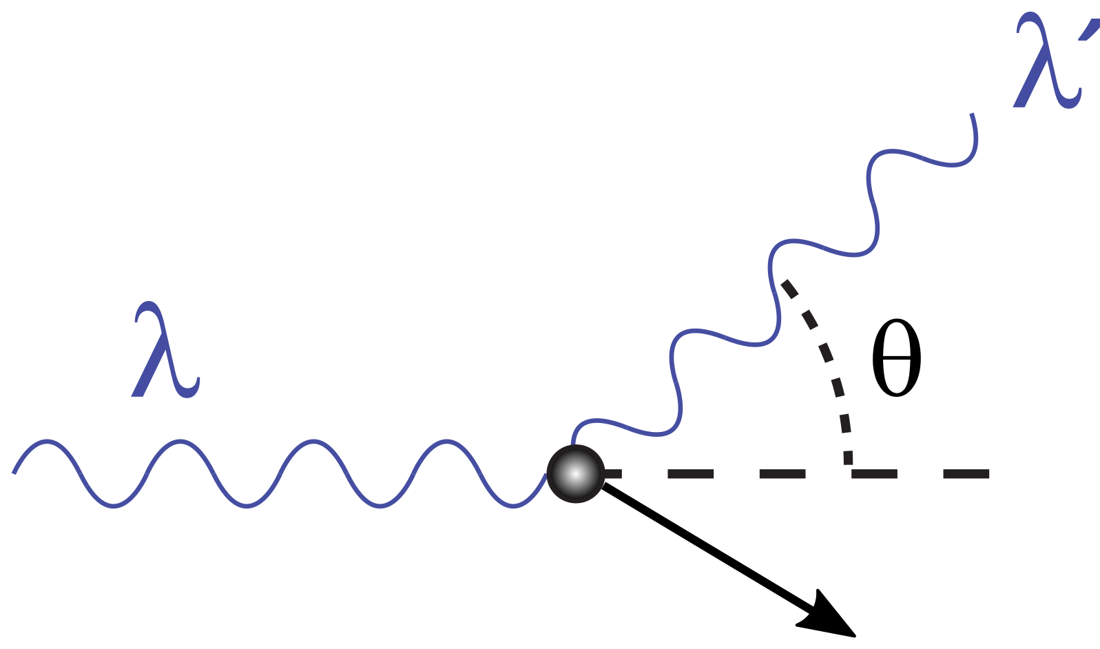
COMPTON SCATTERING
\begin{cases}
E = \sqrt{(pc)^2 + (m_0c^2)^2} = pc \\
E = \hbar \omega \\
p = \frac{E}{c} = \frac{\hbar \omega}{c} = \hbar k
\end{cases}
THE STARSHOT SAIL
A FEW CRACKS STAR SHOWING
DAVISON-GERMER EXPERIMENT
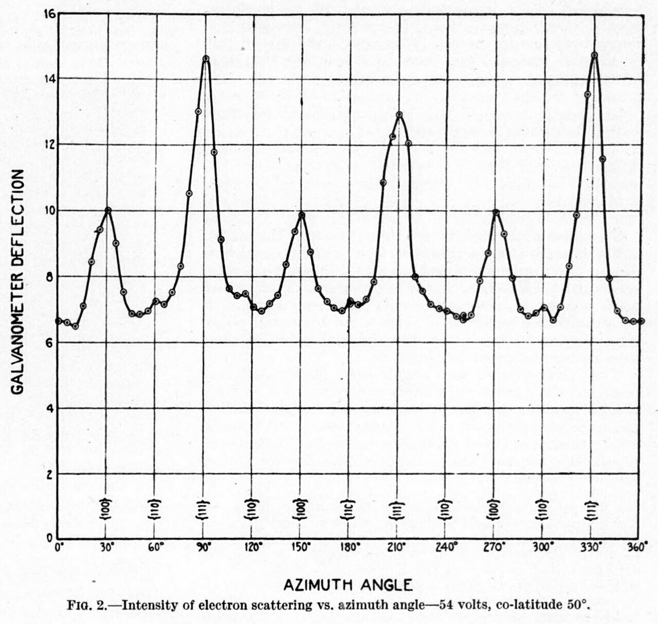
\lambda = \hbar \frac{2 \pi}{p} = \frac{h}{p}
p = \frac{E}{c} = \frac{\hbar \omega}{c} = \hbar k
A FEW CRACKS STAR SHOWING
DAVISON-GERMER EXPERIMENT
THE MATH FRAMEWORK OF QUANTUM MECHANICS
-
State of a quantum system: \(\ket{\psi}\in\mathcal{H} \)
-
Superposition principle: if \(\ket{\psi},\ket{\phi} \in \mathcal{H} \Rightarrow a \ket{\psi} + b\ket{\phi} \in \mathcal{H}\) with \(a,b \in \mathbb{C}\).
-
\(\mathcal{H}\) is a Hilbert space, i.e a complex vector space endowed with an inner product.
-
Inner product: if \(\ket{\psi},\ket{\phi} \in \mathcal{H} \, \Rightarrow \, \braket{\phi|\psi} \in \mathbb{C}\):
-
\(\braket{\phi|\psi}=\braket{\psi|\phi}^*\)
-
\(\braket{\psi|\psi} \in \mathbb{R} \, \forall \ket{\psi}\)
-
For any non-zero vectors \(\braket{\psi|\psi} >0\) and \(\sqrt{\braket{\psi|\psi}}\) is the norm of the vector.
-
Kets representing physical states are normalized: \(\braket{\psi|\psi}=1\).
-
If the inner product of two kets \(\ket{\psi}\) and \(\ket{\phi}\) is zero, \(\braket{\psi|\phi}=0\), they are said to be orthogonal
-
FUNDAMENTALS
THE MATH FRAMEWORK OF QUANTUM MECHANICS
-
Complete orthonormal basis: \( \braket{\phi_m|\phi_n}=\delta_{mn}\) with \(\delta_{mn}=\begin{cases}1 \; m=n \\ 0 \; m \neq n\end{cases}\)
-
Every state may be expressed as : \(\ket{\psi}=\sum_n^d c_n \ket{\phi_n}\), the \(c_n\) coefficients are unique and are the components of \(\ket{\psi}\). d is the dimension of the Hilbert space: \(d=dim\{\mathcal{H}\}\)
-
If \(\ket{\psi}\) is our state, and we associate \(\ket{\phi_k}\) with the kth possible outcome of a measurment, then the probability of the outcome is \(p(k)=|\braket{\phi_k|\psi}|^2\), and we have \(\sum_k p(k) = 1\)
ORTHONORMAL BASIS
THE MATH FRAMEWORK OF QUANTUM MECHANICS
-
A general ket \(\ket{\beta}\) may be represented by the column vector of his coefficients \(\mathbf{b}\).
-
A general bra \(\bra{\alpha}\) may be represented by the Hermitian Conjugate of his coefficients \(\mathbf{a}^{\dag}\). If \(\ket{\alpha}=\sum_n^d a_n\ket{\phi_n}\) then \(\bra{\alpha}=\sum_n^d a_n^{*}\bra{\phi_n}\)
-
A general inner product \(\braket{\alpha|\beta}\), with \(\ket{\alpha}=\sum_n^d a_n \ket{\phi_n}\) and \(\ket{\beta}=\sum_n^d b_n \ket{\phi_n}\) may be then specified through the respective components: \(\braket{\alpha|\beta}=\sum_n^n a_n^* b_n\)
-
The inner product \(\braket{\alpha|\beta}\) then becomes \(\mathbf{a}^{\dag}\mathbf{b}\).
-
\(G:\mathcal{H} \rightarrow \mathcal{H}\) is a linear operator if \(G(a\ket{\psi_1}+b\ket{\psi_1})=a G \ket{\psi_1}+b G \ket{\psi_2}\)
-
If \(\{\ket{\phi_n}\}\) is a complete orthonormal basis and \(\ket{\psi}=\sum_n^d c_n \ket{\phi_n}\) then \(G\ket{\psi}=\sum_n^d c_n G \ket{\phi_n}\)
-
\((AB)\ket{\psi}=A(B\ket{\psi})\) and the commutator is defined as \([A,B]=AB-BA\)
-
\(\ket{\alpha}\bra{\beta}\) is the outer product operator. If \(\{\ket{\phi_n}\}\) is a complete orthonormal basis then \(\sum_n^d \ket{\phi_n}\bra{\phi_n}=\mathbb{1}\) where \(\mathbb{1}\) is the identity operator.
-
If \(\{\ket{\phi_n}\}\) is a complete orthonormal basis, a general linear operator \(G\) may be described by a matrix whose elements are \(G_{mn}=\bra{\phi_m}G\ket{\phi_n}\)
MATRIX REPRESENTATION
THE MATH FRAMEWORK OF QUANTUM MECHANICS
-
An observable A is a basic measurement in which each outcome is associated with a numerical value.
-
If \(\{\ket{\phi_n}\}\) is a complete orthonormal basis associated with the measurements of \(A\), and \(A_n\) is nth outcome of a measurement, then the operator \(A\) associated to A is defined as \(A\ket{\phi_n}=A_n\ket{\phi_n}\)
-
In the measurement basis \(A_{mn}=\bra{\phi_m}A\ket{\phi_n}=A_n\delta_{mn}\) yields a diagonal matrix with \(A=\sum_n^d A_n \ket{\phi_n}\bra{\phi_n}\).
-
Given the state \(\ket{\psi}\), where the nth outcome happens with probability \(p(n)=|\braket{\phi_n|\psi}|^2\), the expectation value \(\langle A \rangle\) is:
-
\( \langle A \rangle=\sum_n^d p(n) A_n \)
-
\( \langle A \rangle=\bra{\psi}A\ket{\psi} \)
-
\( \langle A \rangle=\bm{\psi}^{\dagger}\mathbf{A}\bm{\psi} \)
-
-
Given an operator \(A\) on \(\mathcal{H}\) its adjoint, or Hermitian Conjugate \(A^{\dagger}\) is defined so that, \(\forall \, \ket{\alpha},\ket{\beta} \in \mathcal{H} \), we have \(\bra{\alpha}A^{\dagger}\ket{\beta}=(\bra{\beta}A\ket{\alpha})^* \)
-
\(A=(A^{\dagger})^{\dagger}\)
-
\((AB)^{\dagger}=B^{\dagger}A^{\dagger}\)
-
\((A^{\dagger})_{mn}=A_{nm}^*\)
-
An Hermitian operator satisfies \(A^{\dagger}=A\), therefore \(\langle A \rangle=\bra{\psi}A\ket{\psi}\) is always real. Our observables are real valued and represented by Hermitian operators.
-
The eigenvectors of an Hermitian operator \(A\), represented by \(\ket{\alpha_n}\) form a complete orthonormal basis of \(\mathcal{H}\).
-
OBSERVABLES
DISCRETE VS CONTINUUM PROBABILITY
-N
N
-L
L
\begin{cases}
x_k=k \Delta x \\
L=N \Delta x
\end{cases}
\begin{cases}
l=unit \, length \\
\Delta x = \frac{l}{\sqrt{N}}
\end{cases}
N \rightarrow \infty
\overbrace{}
l
\mathrm{Pr}(k=n)=p_N(n)
\mathrm{Pr}(x_k \in [a,b]) = \sum_{x_k \in [a,b]} \mathcal{P}_N(x_k) \Delta x
\mathrm{Pr}(x \in [a,b]) =\int_{a}^{b} \mathcal{P}(x)dx
OUTCOME PROBABILITY
EXPECTATION VALUE
\langle F \rangle =\sum_k F(x_k)p_N(k)
\langle F \rangle =\sum_k F(x_k)\mathcal{P}_N(k) \Delta x
\langle F \rangle = \int_{-\infty}^{\infty}F(x)\mathcal{P}(x)dx
\sum_{k=-N}^{k=N} p_N(k) = 1
\sum_{x_k=-L}^{x_k=L} \mathcal{P}_N(x_k) \Delta x= 1
\int_{-\infty}^{\infty} \mathcal{P}(x)dx = 1
PROBABILITY NORMALIZATION
p_N(k)
\mathcal{P}(x_k)= \frac{p_N(k)}{\Delta x}
\mathcal{P}(x)
PROBABILITY DISTRIBUTION
DISCRETE VS CONTINUUM STATES
-N
N
-L
L
\begin{cases}
x_k=k \Delta x \\
L=N \Delta x
\end{cases}
\begin{cases}
l=unit \, length \\
\Delta x = \frac{l}{\sqrt{N}}
\end{cases}
N \rightarrow \infty
\overbrace{}
l
\mathrm{Pr}(x_k \in [a,b]) = \sum_{x_k \in [a,b]} \braket{\psi_N|x_k}\ket{x_k} \Delta x
\mathrm{Pr}(x \in [a,b]) =\int_{a}^{b} |\psi(x)|^2dx
OUTCOME PROBABILITY
\mathrm{Pr}(k=n)=|\braket{\psi_N|\phi_n}|^2
\ket{\phi_k}
\ket{x_k}= \frac{\ket{\phi_k}}{\Delta x}
\ket{x}
ORTHONORMAL BASIS
\ket{\psi_n}=\sum_k \braket{\phi_k|\psi_N}\ket{\phi_k}
\ket{\psi_N} = \sum_{x_k=-L}^{x_k=L} \psi_N(x_k)\ket{x_k}\Delta x;\, \psi_N(x_k)=\braket{x_k|\psi_N}
\ket{\psi} = \int_{-\infty}^{\infty} \psi(x) \ket{x} dx
PHYSICAL STATE
DISCRETE VS CONTINUUM STATES
\int_{-\infty}^{\infty}|\psi(x)|^2 dx =1
Normalization:
\mathcal{P}(x) = |\psi(x)|^2
Probability Density:
\int_{-\infty}^{\infty}\ket{x}\bra{x} dx =\mathbb{1}
Identity Matrix:
\braket{\phi|\psi}=\int_{-\infty}^{\infty}\phi(x)^*\psi(x) dx
Inner product:
\braket{x|x'}=\delta(x-x'); \; \int_{-\infty}^{\infty} \braket{x|x'} dx = 1
Orthonormality:
\delta(x-x')
Dirac's delta:
DISCRETE VS CONTINUUM LINEAR OPERATORS
G(a\ket{\phi}+b\ket{\psi})=aG(\ket{\phi})+bG(\ket{\psi})
\frac{d}{dx}\big[a\phi(x)+b\psi{x}\big]=a\frac{d[\phi(x)]}{dx} + b\frac{d[\psi(x)]}{dx}
HERMITIAN OPERATORS AND OBSERVABLES
-N
N
\overbrace{}
l
-L
L
G \ket{\phi_n}=G_n \ket{\phi_n}
\langle G \rangle= \bra{\psi}G\ket{\psi}
G
G = (G_{mn})
G(\alpha\mathbf{a}+\beta\mathbf{b})=\alpha G \mathbf{a} + \beta G \mathbf{b}
\langle G \rangle=\bm{\psi}^{\dagger}\mathbf{G}\bm{\psi}
G_n=G_{mn}\delta_{mn}=\bm{\phi_m}^{\dagger}\mathbf{G}\bm{\phi_n}
G = \frac{d}{dx}
\frac{d[\phi(x)]}{dx} = g \phi(x)
\langle G \rangle= \int_{-\infty}^{\infty}\psi^*(x)\big[\frac{d}{dx}\big] \psi_n(x)dx
ABSTRACT
DISCRETE REPRESENTATION
(\mathcal{H},\braket{\psi|\phi})
\ket{\alpha}
\bm{\chi}
\ket{\chi}
\ket{\psi}
\ket{\phi}
a\ket{\phi} + b\ket{\phi}
\{\ket{\phi_n}\}
(\mathbb{C}^n,\bm{\phi}^{\dagger}\bm{\psi})
\bm{\psi}
\bm{\xi}
\bm{\alpha}
\bm{\phi}
a\bm{\psi}+b\bm{\phi}
G
A
B
G
A
B
(G_{mn})
(A_{mn})
(B_{mn})
\braket{\phi|\psi}
A^{\dagger}=A
\mathbb{R,C}
CONTINUOUS REPRESENTATION
(\mathcal{H},\braket{\psi|\phi})
\ket{\alpha}
\chi(x)
\ket{\chi}
\ket{\psi}
\ket{\phi}
a\ket{\phi} + b\ket{\phi}
\{\ket{x}\}
\bigg(\mathcal{L}_2,\int_{-\infty}^{\infty}\psi^*(x)\phi(x)dx \bigg)
\psi(x)
\xi(x)
\alpha(x)
\phi(x)
a\psi(x)+b\phi(x)
G
A
B
G
A
B
x
\frac{d}{dx}
\int dx
\braket{\phi|\psi}
A^{\dagger}=A
\mathbb{R,C}
FIRST POSTULATE OF QUANTUM MECHANICS
This function is called the wavefunction and has the property that \( \psi(x,t)^*\psi(x,t) dx \) is the probability that the p article lies in the volume element \(dx\) located at \(x\) and time \(t\)
\psi(x,t)
The state of a quantum mechanical system is completely specified by the function \( \psi(x,t) \) that depends on the coordinates of the particle \( x\) and the time \( t\)
\begin{cases}
P(x,t) = |\psi(x,t)|^2 \\
|\psi(x,t)|^2 = \psi(x,t)^*\psi(x,t)
\end{cases}
WAVEFUNCTION
PROBABILITY DENSITY
\int_{-\infty}^{\infty}|\psi(x,t)|^2 dx = 1
NORMALIZATION
SCHROEDINGER EQUATION
If we represent a free particle as a plane wave, we can intuitively illustrate the rationale behind the postulation of Schröedinger equation.
A NON-RIGOROUS BUT INTUITIVE INTRODUCTION
\psi(x,t)= e^{i(kx - \omega t)}
\frac{-\hbar^2}{2 m} \frac{\partial^2}{\partial x^2}\psi(x,t) + U(x,t)\psi(x,t)=ih \frac{\partial}{\partial t}\psi(x,t)
To every observable in classical mechanics there corresponds a linear Hermitian operator in quantum mechanics.
SECOND POSTULATE OF QUANTUM MECHANICS
- \(\hat{x} \; \Rightarrow \; x \; \Rightarrow \; \mathbf{r}\)
- \(\hat{p} \; \Rightarrow \; -i \hbar \frac{\partial}{\partial x} \; \Rightarrow \; -i \hbar \vec{\nabla}\)
- \(\hat{T} \; \Rightarrow \; - \frac{\hbar^2}{2m} \frac{\partial^2}{\partial x^2} \; \Rightarrow \; -\frac{\hbar^2}{2m}\nabla^2\)
- \(\hat{U} \; \Rightarrow \; U(x) \; \Rightarrow \; U(\mathbf{r}) \)
- \(\hat{H} \; \Rightarrow \; - \frac{\hbar^2}{2m} \frac{\partial^2}{\partial x^2} + U(x) \; \Rightarrow \; -\frac{\hbar^2}{2m}\nabla^2 +U(\mathbf{r})\)
- \(\hat{L}_x \; \Rightarrow \; -ih(y\frac{\partial}{\partial z} - z \frac{\partial}{\partial y})\)
- \(\hat{L}_y \; \Rightarrow \; -ih(z\frac{\partial}{\partial x} - x \frac{\partial}{\partial z})\)
- \(\hat{L}_z \; \Rightarrow \; -ih(x\frac{\partial}{\partial y} - y \frac{\partial}{\partial x})\)
- \(\hat{f} \; \Rightarrow \; f(x,\hat{p},t) \; \Rightarrow \; f(\mathbf{r},\hat{p},t) \)
TIME INDEPENDENT SCHRÖDINGER EQUATION
\hat{H} = -\frac{\hbar^2}{2 m} \nabla^2 + U(\mathbf{r}) \; \Rightarrow \; \psi(\mathbf{r},t) = \varphi(\mathbf{r})\xi(t)
\begin{cases}
\hat{H} \varphi(\mathbf{r}) = E\varphi(\mathbf{r}) \\
\\
i \hbar \frac{d \xi(t)}{dt} = E \xi(t)
\end{cases}
A FEW EXAMPLES IN ONE DIMENSION
\bigg[-\frac{\hbar^2}{2 m} \frac{\partial^2}{\partial x^2} + U(x)\bigg]\varphi(x)=E \varphi(x)
Materials and Platforms for AI - Introduction to Quantum Mechanics
By Giovanni Pellegrini


