onde
introduzione alle onde longitudinali
onde trasversali e longitudinali
onde trasversali
onde longitudinali

cenni di proprietà elastiche dei materiali
modulo di young (E)
deformazione longitudinale
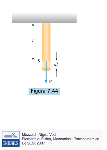
\[ \frac{F}{S} = E \frac{\Delta l}{l} \]
\[ \Downarrow \]
\[ F = k \, \Delta x \]
\[ F = \left( \frac{E \, S}{l} \right) \Delta l \]
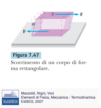
modulo di taglio (G)
deformazione di taglio
\[ \frac{F}{S} = G \frac{\Delta x}{l} \]
\[ \Downarrow \]
\[ F = k \, \Delta x \]
\[ F = \left( \frac{G \, S}{l} \right) \Delta x \]
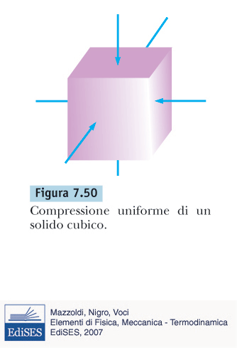
modulo di compressibilità (B)
deformazione di volume
\[ \Delta P = B \frac{\Delta V}{V} \]
modulo di compressibilità
gas ideale a temperatura costante
\[ P V = n R T \]
\[(P + \Delta P) (V + \Delta V) = n R T \]
\[ \Downarrow \]
\[ P V = (P + \Delta P) (V + \Delta V) \]
\[ \Downarrow \]
\[ \frac{\Delta P}{P} = -\frac{\Delta V}{V}; \; \Delta P = - B \frac{\Delta V}{V} \]
\[ \Downarrow \]
\[ \boxed{B = P} \]
velocità di un'onda

corda tesa
barra metallica
gas
\[ v = \sqrt{\frac{T}{\mu}} \]
\[ v = \sqrt{\frac{E}{\rho}} \]
\[ v = \sqrt{\frac{P}{\rho}} = \sqrt{\frac{B}{\rho}} \]
PIPISTRELLI, DENSITÀ DELL'ARIA E VELOCITÀ DEL SUONO
\[ v_{aria} = \sqrt{\frac{P_{atm}}{\rho_{aria}}} \approx 300 \, m/s \]
\[ v_{elio} = \sqrt{\frac{P_{atm}}{\rho_{elio}}} \approx 800 \, m/s \]
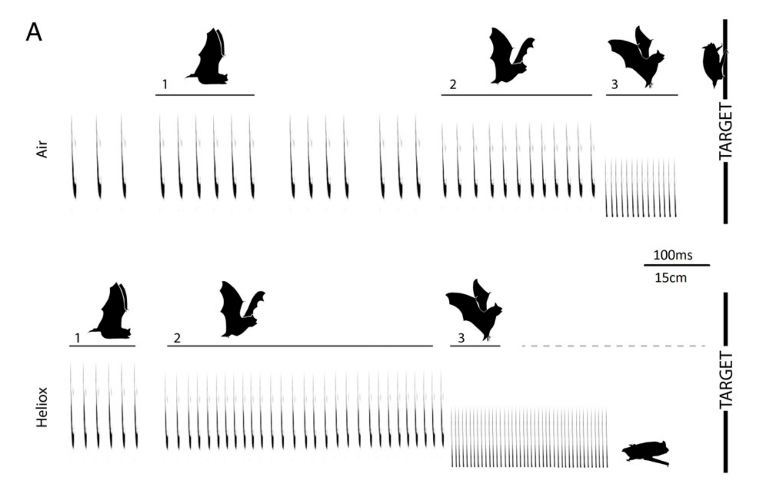
effetti della densità del mezzo
elio
esafluoruro di zolfo
onde longitudinali sinusoidali
\[ s(x,t) = s_{m} cos(k x - \omega t) \]
\[ \Delta P(x,t) = \Delta P_{m} sin(k x - \omega t) \]
interferenza tra onde sinusoidali
\[ s_{1}(x,t) = s_{m} cos(kx - \omega t) \]
\[ s_{2}(x,t) = s_{m} cos(kx - \omega t + \phi) \]
\[ \boxed{y(x,y) = s_{1}(x,t) + s_{2}(x,t) = 2 s_{m} cos \left( \frac{\phi}{2} \right) cos \left( kx - \omega t + \frac{\phi}{2} \right)} \]
\[ \Downarrow \]
intensità di un'onda
\[ I = \frac{P}{S} \; [W/m^2] \]
\[ I = \frac{1}{2} \, \rho \, v_{onda} \, \omega^{2} \, s_{m}^{2} \]
\[ \beta = 10 \cdot log \left( \frac{I}{I_{0}} \right); \; I_{0} = 10^{-12} W/m^{2} \]
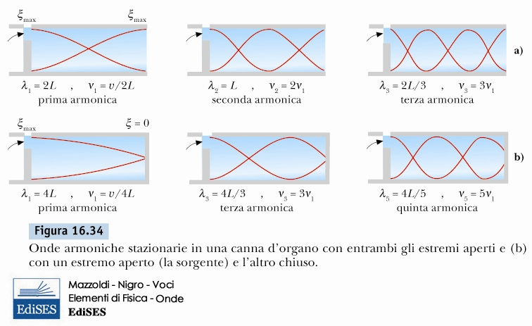
interferenza, onde stazionerie e risonanze
\[ s_{1}(x,t) = s_{m} cos(kx - \omega t) \]
\[ s_{2}(x,t) = s_{m} cos(kx + \omega t) \]
\[ s(x,t) = s_{1}(x,t) + s_{2}(x,t) \]
\( \Downarrow \)
\[ \boxed{s(x,t) = [ 2 s_{m} cos(kx) ] cos( \omega t)} \]
\[ \boxed{ \lambda = \frac{2 L}{n}; \; n=1,2,3... \; due \, aperture} \]
\[ \boxed{ \lambda = \frac{4 L}{n}; \; n=1,3,5... \; due \, aperture} \]
battimenti
\[ s_{1}(t) = s_{m} cos(\omega_{1} t) \]
\[ s_{2}(t) = s_{m} cos(\omega_{2} t) \]
\[ s(t) = s_{1}(t) + s_{2}( t) \]
\[ \Downarrow \]
\[s(t) = [2 s_{m} cos(\omega_{a} t)] cos(\omega_{b} t) \]
\[ \omega_{a} = \frac{1}{2}(\omega_{1}-\omega_{2}) \]
\[ \omega_{b} = \frac{1}{2}(\omega_{1}+\omega_{2}) \]
Musicologia: onde longitudinali
By Giovanni Pellegrini


