Machine Learning Basics
Deep Learning Book - Ch 5
Disclaimer
There is math.
There is theory.
There is pseudocode.
A lot of content in 60min
Interact with us!
"M.L. is easy!11!"
"M.L. is easy!11!"
I'm Hanneli
I'm Gustavo
Goals
- Go over the main topics of Ch. 5
- Connect the missing pieces
- Show the relation between ML theory, Statistics and implementation
Agenda
- Definition of "Learning Algorithm" (Gustavo)
- Application examples (Gustavo)
- Linear Regression demystified (Hanneli)
- Factors for the success of a learning algorithm (Hanneli)
- Useful concepts from Statistics (Gustavo)
- Code time - examples with Octave/Python (Hanneli)
- Extras and References
General idea
Training set
Learning Algorithm
hypothesis
input
predicted output
General Idea
Training set
Learning Algorithm
hypothesis
input
predicted output
What do we
mean by that?
Learning Algorithm
"A program learns from an experience E with respect to some class of tasks T and performance measure P, if P at T improves with E"

T - Task
How a ML system should perform an example
Example - Collection of features (quantitative measured)
- Classification (tag people)
- Transcription (speech recognition)
- Machine Translation (translate)
- Structured output (natural lang)
- Anomaly detection (flag atypical)
- Synthesis (video game textures)
- Denoising (predict clean example)
P - Performance Measure
Quantitative performance measure of the algorithm
Factors
a) Accuracy
b) Error Rate
P is specific to a task T
E - Experience
Kind of experience during the learning process
Supervised Learning
Unsupervised Learning
Reinforcement Learning
We have an idea of the right answer for what we are asking. Example: Given a picture of a person, predict how old is he/she
We have no idea of the right answer for what we are asking. Example: Given a collection of items you don't know, try to group them by similarity.
Let the machine take control of the context and you provide input feedback.
Example: Reduce items in stock by creating dynamic promotions
Problem:
Sell used cars. Find the best price to sell them (not considering people who collect old cars)
Do we have any idea for know relations?
older -> cheaper
unpopular brands -> cheaper
too many kms -> cheaper
Problem:
Sell used cars. Find the best price to sell them (not considering people who collect old cars)
What kind of M.L. Algorithm would you use here? (E)
Supervised Learning
Algorithm draft:
Chose one variable to analyse vs what you want to predict (example: year x price). Price is the variable you want to set a prediction. (T)
Come up with a training set to analyse these variables
Number of training examples (m)

input variable or features - x
output variable or target - y
Back to the principle
Training set
Learning Algorithm
hypothesis
input
predicted output
m
x
h
y
Strategy to h

Strategy to h
Linear equation
h = ax + b
How do you choose a and b?
From the training set, we have expected values y for a certain x:
Come up with a hypothesis that gives you
the smallest error for all the training set:
The algorithm
h(x)
y
Your hypothesis
for an input x
The output of the training set
-
Measure the difference
The algorithm
h(x)
y
Your hypothesis
for an input x
The output of the training set
-
Measure the difference
for the entire training set (P)
The algorithm
Your hypothesis
for an input x
The output of the training set
-
Measure the difference
for the entire training set
(
)
The algorithm
Your hypothesis
for an input x
The output of the training set
-
We don't want to cancel positive and negative values
Average
Mean Square Erros (MSE)
The algorithm
-
Cost Function
J =
We want to minimize the difference
Understanding it

Understanding it

We can come up with different hypothesis (slopes for h function)
Understanding it

We can come up with different hypothesis (slopes for h function)
Understanding it

That's the difference
for a certain cost function
Understanding it
That's the difference
for another cost function

This cost function (J) will be a parabola

Minimum value
on h = ax +b,
we are varying a
J(a)
We also need to vary b. J will be a surface (3 dimensions)
h = ax + b
J(a,b)
Back to the algorithm
Minimize any Cost Function.

plotted in Jan/17
Back to the algorithm
Minimize any Cost Function.

Min
We start with a guess
And 'walk' to the min value
Back to the algorithm
Or:

Min
How do you find the min values of a function?
Calculus is useful here

Calculus - we can get this information from the derivative
Remember: we start with a guess and walk to the min value
Back to the cost function
Towards the min value
We start with
a guess
Walk on
the
graph
Partial Derivatives
Gradient Descent
Partial derivatives
(min value)
We start with
a guess
Walk on
the
graph
Back to the cost function
Learning rate
(another guess)
Repeat until convergence
Going back to used cars
We are only analysing year vs price. We have more factors: model, how much the car was used before, etc
Back to the principle
Training set
Learning Algorithm
hypothesis
input
predicted output
m
x
h
Strategy to h
Consider multiple variables: a, b, c,... (or using greek letters)
Can you suggest the next steps?
Gradient Descent for multiple Variables
Repeat until convergence
Multiple Variables
We can rewrite this as
Predicted
Output
Parameters
Vector
Input
Vector
(how did we get here?)
Adjusting the names
Recap
- Hypothesis h
- Cost function: the difference between our hypothesis and the output in the training set
- Gradient descent: minimizes the difference
Don't forget this :)
Problem
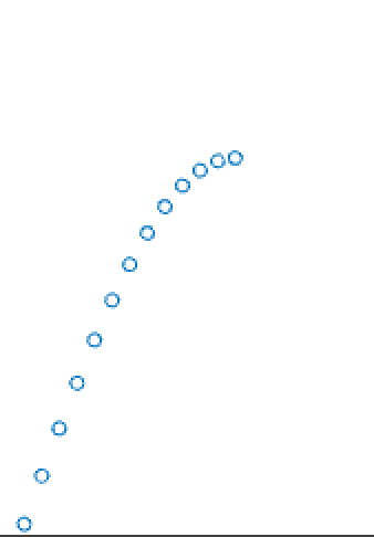
Problem

Does it look good?
Underfitting

The predicted output is not even fitting the training data!
Problem
Does it look good?
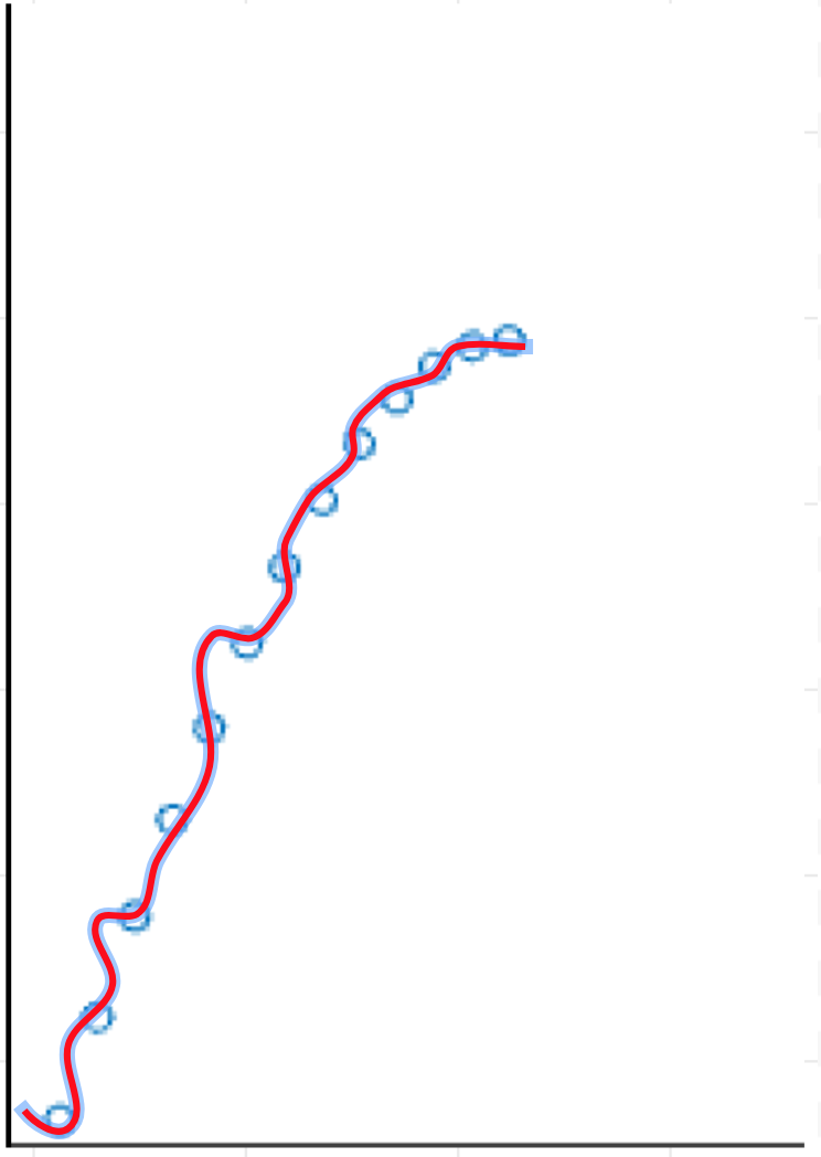
Overfitting
The model fits everything

[Over, Under]fitting were problems related to the capacity
Capacity: Ability to fit a wide variety of functions
Overfitting
Underfitting
How can we control the capacity?
a) change the number of input features
b) change the parameters associated with the features
By controlling the capacity, we are searching for an ideal model
It is difficult to know the true probability distribution that generates the data, so we want the lowest possible error rate (Bayes error)
Problem
The training set works fine; new predictions are terrible
The problem might be the cost function (comparing the predicted values with the training set)
-
J =
A better cost function
-
J =
Regularization param
It controls the tradeoff / lowers the variance
c) Regularization
(another mechanism to control the capacity)
d) Hyperparameters - parameters that control parameters
Select setting that the algorithms can't learn to be hyperparameters
Question: If we use the entire dataset to train the model, how do we know if it's [under,over]fitting?
Your Dataset
Training set
Learn the parameter θ; compute J(θ)
Test set
Compute the test set error (identify [under,over]fitting)
70%
30%
(cross-validation)
We can analyze the relations between the errors on the training and test sets
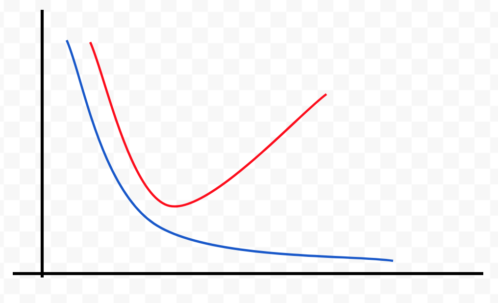
Error
Capacity
J(θ) test error
J(θ) train error

Error
Capacity
J(θ) test error
J(θ) train error
Bias problem (underfitting)
J(θ) train error is high
J(θ) train ≈ J(θ) test
J(θ) train error is low
J(θ) test >> J(θ) train
Variance problem (overfitting)
Bias - measures the expected deviation from the true value of the function or parameter
Variance - measures the deviation from the expected estimator value that any sampling can cause
How do we select good estimators?
A: Maximum likelihood estimation or Bayesian statistics
WE MADE IT TO THE END OF THIS SESSION!

(Not yet!)
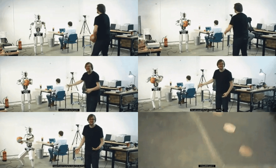
How do I transform all this into code???

Octave/ Matlab for prototyping
Adjust your theory to work with Linear Algebra and Matrices
Expand the derivatives:
Repeat until convergence
The dataset:
source: https://github.com/stedy/Machine-Learning-with-R-datasets/blob/master/usedcars.csv

The code in Octave
data = load('used_cars.csv'); %year x price
y = data(:, 2);
X = [ones(m, 1), data(:,1)];
theta = zeros(2, 1); %linear function
iterations = 1500;
alpha = 0.01;
m = length(y);
J = 0;

predictions = X*theta;

sqErrors = (predictions - y).^2;
J = 1/(2*m) * sum(sqErrors);

J_history = zeros(iterations, 1);

for iter = 1:iterations
    x = X(:,2);
    delta = theta(1) + (theta(2)*x);
    tz = theta(1) - alpha * (1/m) * sum(delta-y);
    t1 = theta(2) - alpha * (1/m) * sum((delta - y) .* x);
    theta = [tz; t1];
    J_history(iter) = computeCost(X, y, theta);
end
Initialise
Cost
Function
Gradient
Descent

In a large project
Linear regression with C++
mlpack_linear_regression --training_file used_cars.csv
 --test_file used_cars_test.csv -v
Bonus!
References
- Coursera Stanford course
- Awesome M.L. Books
- Alex Smola and S.V.N. Vishwanathan - Introduction to Machine Learning
- mlpack
- scikit-learn
- MILA classes
GIF time

Thank you :)
Questions?
gustavoergalves@gmail.com
hannelita@gmail.com
@hannelita

Machine Learning Basics
By Hanneli Tavante (hannelita)
Machine Learning Basics
Deep Learning Book - Ch 5
- 2,025


