Real-world decision making through MABs and multi-level reinforcement learning on agent-based models
Harshavardhan Kamarthi
Presented at Data Seminar (Oct 8)
AI Economist
- Learn optimal tax policies
- Hard to experiment in real-world
- Lucas critique
- Fine-grained modeling of behavior
- Ad-hoc, homogenous behavior rules
- Flexible objectives and free parameters
- easy to add or remove policy, action constraints
- Learn directly from observations
- Use experience from agents and planners to optimize
- calibrate (macro) parameters from real-world data
Zheng et al
AI Economist for Tax Policies
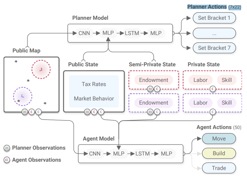
- Agent-based model: Gather-Build-Trade
- Each agent maximizes its own utility by
- Gathering resources
- Building houses
- Trading resources and houses for coins
- High-level social planner
- Levies tax on income
- Redistributes the collected tax to everyone equally

Environment
- 25 x 25 grid world
- Each grid
- Source cell: can spawn new resources stochastically
- House cell: occupied by owner only
- Water cell: can not be occupied
- Other cells
- Building: need one unit of stone and wood to build a house
- Trading:
- Continuous double auction
- Buy and sell resources
- Bracketed tax rate is levied for income earned as determined by planner
Agent State
- Skills (Fixed)
- Gathering skill (0-3)
- Building skill (0-3)
- Resources
- Wood, stone
- Coins
- Trades
- Current ask bids (up to 5)
- Current buy bids (up to 5)
- Location and surroundings (10x10 neighborhood)
- Current tax rate
Agent Actions
- Move actions (UDLR, No-op)
- Build action (Y/N)
- Get coins = (1+Building skill)
- Gather action (if in source cell)
- If available get 1 + (Gathering skill) resources (stochastic)
- Trade
- Add an ask/buy bid for any of the resources
- Can add almost 5 bids per resources
Planner State
- The full map of all agents' locations
- Current tax rate
- All bids in market
- Resources and coins of all agents
Planner Action
- Tax rate for each of the 7 tax brackets
Model
- Tax rate for each of the 7 tax brackets
Agent Reward
- Utility
- Increases with number of coins
- decreases with labor (moving, gathering, trading)
u_i(x_i,l_i) = crra(x_i) - l_i,\ crra(x) = \frac{x_i^{1-\eta - 1}}{1-\eta}
- Consider decreasing marginal return over coins gathered
- Goal: maximize marginal utility at each time step
E[\sum_{t=1}^T (\gamma_t u_{i,t} - u_{i, t-1}) + u_{i,0}]
Planner Reward
- Tradeoff between equality and productivity
- Equality: Gini-index over all post-tax income
- Productivity: total wealth in economy
- Reward:
swf_t = eq_t \times prod_t
E[\sum_{t=1}^T (\gamma_t swf_{t} - swf_{t-1}) + swf_{0}]
- Goal: maximize marginal social welfare
RL Training
- Two level training
- Hard:
- Reward function of agents depends on action of the planner
- Reward function of planner depends of agent policies
- MDPs are unstable
- Tricks: Pre-train agents, Curriculum learning, Entropy regularization
- Pre-train agents:
- Pre train agent networks with random fixed tax policies before joint training
- Curriculum learning: slowly increase variation in tax policies
- Slowly increase the maximum tax rate for planner
- Entropy regularization: improve stochasticity and exploration
Baselines
- Agents' initial position - uniformly at random
- Build, gather skills - Pareto distribution
- Tax rate changes every 20 time steps
Initialization
- No Taxes! (Free market)
- US federal rate (Make brackets s.t USD rates proportional to coins)
- Saez tax policy (optimal with homogenous assumptions on tax elasticity)
Results
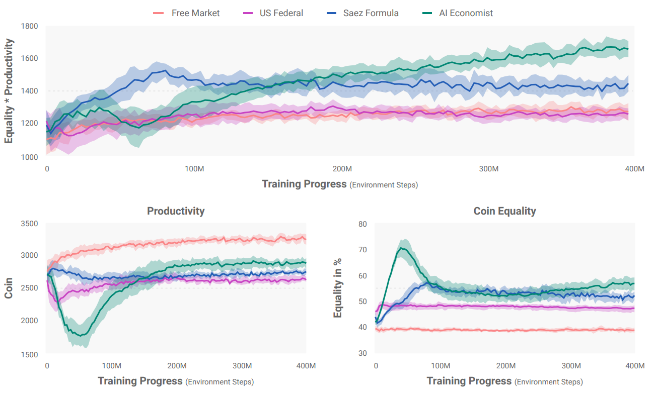
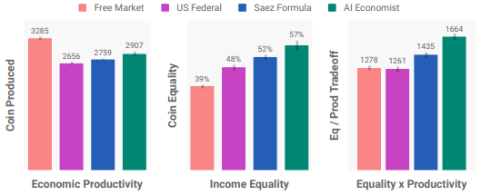
Results
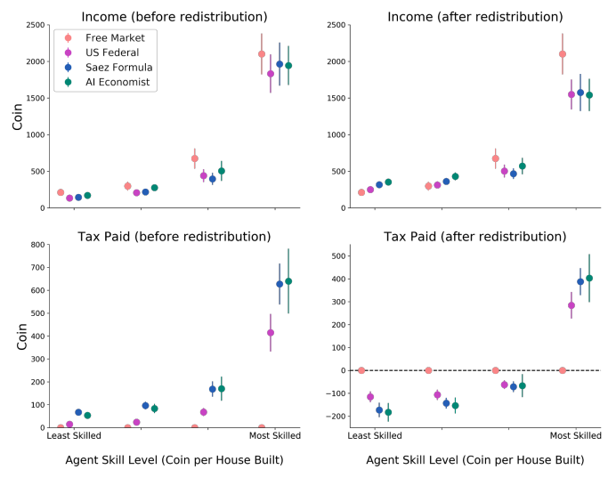
- AI Econ. improves on the best baseline by 16%
- 47% better equality than the free market at cost of only 11% decrease in productivity
- Between progressive and regressive tax structure
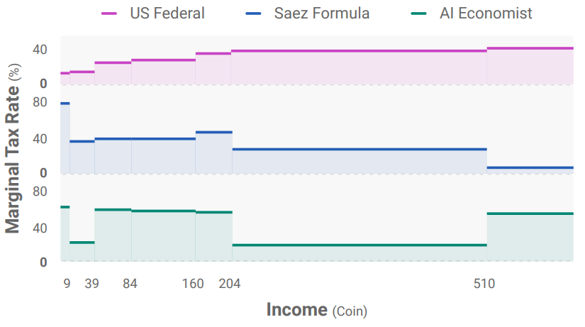
Effect of planner on agent behavior
- Regressive Saez policy makes builders trade less, making them collect resources on their own
- Trading helps redistribute wealth (low tax on gatherers + more time to build)
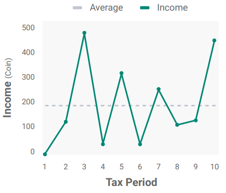
- Gaming the system: initially as planner is converging to optimal policy, agents also alternate total income earned to reduce taxes

What about human participants?
- Used human participants instead of agents to play the game.
- Incentives proportional total income earned at end of the game.

Optimizing Public Health and economy during the pandemic
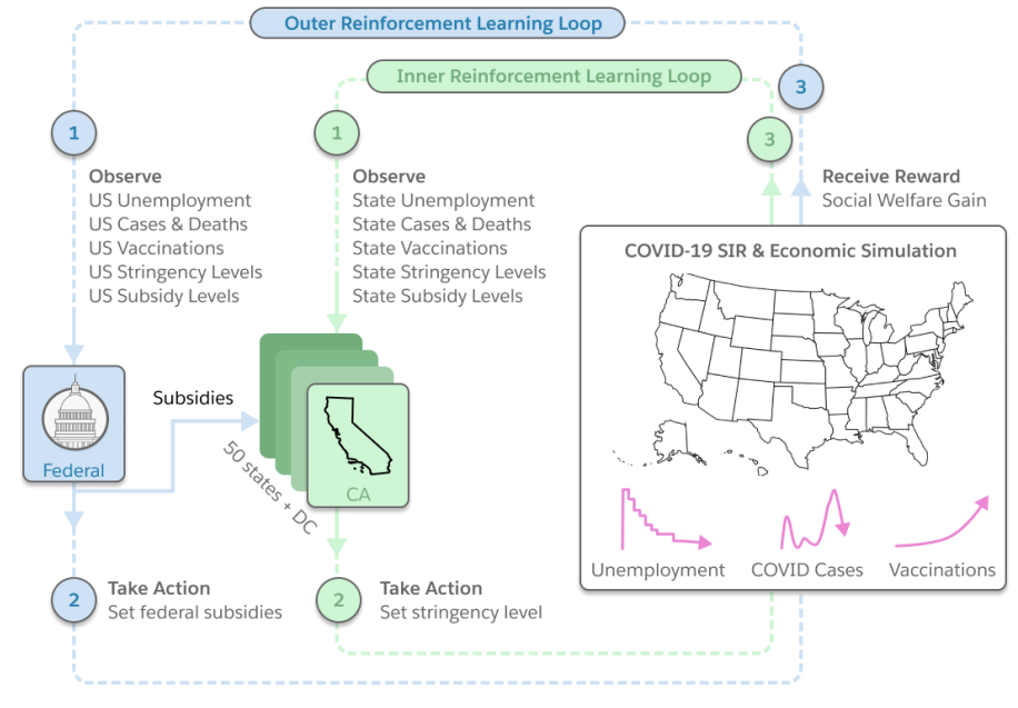
- Analyze and learn policies at Federal and State level
- Federal (planner):
- Provide subsidies to states
- Optimize social welfare
- State: Maximize state level utilities
Optimizing Public Health and economy during the pandemic
Optimizing Public Health and economy during the pandemic

State Level Epidemic Model
- uses a variant of SIR model that accounts for vaccination
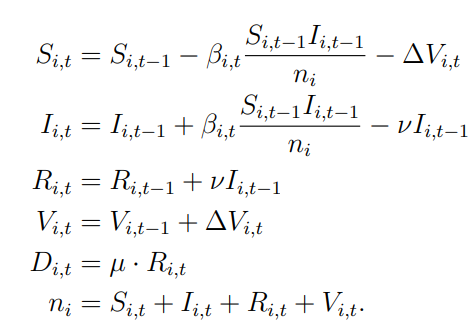
- Transmission rate is location and time specific based on stringency level
- Vaccination rate proportional to population
\beta_{i,t} = \beta_i^{\pi} \pi_{i,t-d} + \beta_0
\Delta V_i = v_i n_i
State Level Econ. Model
- Unemployment proportional to stringency level
U_{i,t} = \text{softplus}\left( \sum_{k=1}^K w_{i,k} \tilde{U}_{i,t}^k \right) + U_i^0
\tilde{U}_{i,t}^k = \sum_{t'=t-L}^t e^{(t'-t)/\lambda_k} \Delta\pi_{i,t'}
- Economic output depends on available workers and federal subsidies
\omega_{i,t} = c(n_i - D_{i,t} - \eta I_{i,t}) - U_{i,t}\\
P_{i,t} = k\omega_{i,t} + T_{i,t}
Rewards
- Condiser health index and economic productivity
r_{i,t} = \alpha_i \Delta H_i + (1-\alpha_i) \Delta E_i\\
\Delta H_{i,t} = - \Delta D_{i,t}\\
\Delta E_{i,t} = crra\left( \frac{P_{i,t}}{P_i^0}\right)
- At federal level aggregate state-level productivity except penalize for subsidies
P_{f,t} = \sum_{i} P_{i,t} - c T_{i,t}
Action and policy parametrization

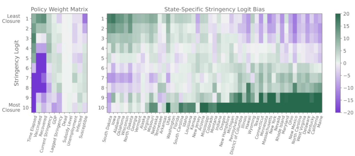
- Log-linear policies.
- Interpretability over weights (same for all states) and bias (each state)
- Discretize to 10 levels of stringency
- 20 levels of subsidies
- Actual subsidy proportional to population of state
Calibration
Datasets
- Covid-19 Govt. policy Tracker: Stringency
- Covid-19 Money Tracker - subsidies
- JHU death estimates - Deaths
- Daily unemployment - BLS
parameters to calibrate
- Death rate, vaccination rate(state), recovery rate
- Baseline params: infection, unemployment, productivity
- State level
\alpha_i
Results

- Simulation from March 22 2020 to April 30 2021
- Calibration fits well with real world
- AI imposes higher stringency
- But unemployment is usually larger
Results
- 4.7% higher federal welfare (reward)
- Better balance between unemployment and deaths (?)
- Much lower subsidies ($35B vs $630B)

Results
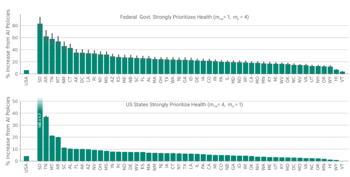
- Changing priority factor to focus more on health, AI econ does even better.
Interpretability
- Effect on individual features on stringency
- State-wise bias on stringency
RL for border testing policies
- Leverage demographic features from travelers to provide estimates of infection prevalence
- Use prevalence estimates to better sample travelers for testing
- Deployed in real world - 40 Ports of entry in Greece
Bastani et al
Traveller data
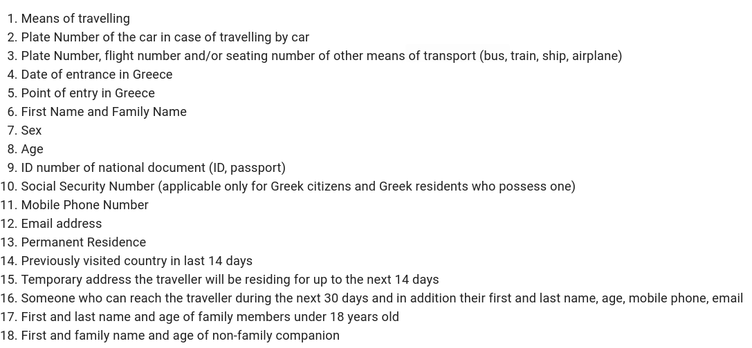
- Used anonymized categorical features: Country, Region, Age, Gender
- Used Lasso regularize on past data to predict positive case to select important features
- This determines classes of travellers for test allocation
Problem
- Allocate tests to each type for day t
- Subject to:
- Total budget for tests
- Assume is probability of bing positive for class k
T_k(t)
R_k(t)
max \sum_t \sum_k T_k(t) R_k(t)
But:
- Prevalence probability is unknown
- May Change
- We need to decide since day 0
- Allocate higher tests for those whose estimates are high
- Allocate tests to classes for which we have low certainty
- Exploit vs Explore Dilemma
Estimation
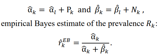
- Use empirical Bayes to estimate new prevalence based on past 14 days cases
- Use a Beta prior: the prior parameters for all classes of same country is same (weight sharing)
Allocation
- Recall: Explore vs Exploit dilemma
- Use Multi Arm Bandits
- Specifically used modified version of Optimistic Gittins Index
- Good guarantees for batched decision making
- Similar motivation to UCB methods (Optimism in face of uncertainty)
Results
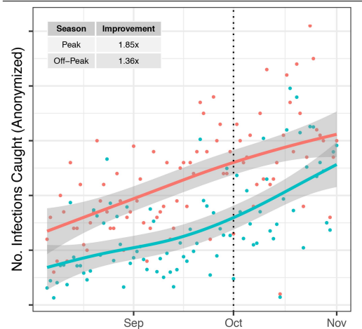
- 54.7% better than random allocation (73% during Oct peak)
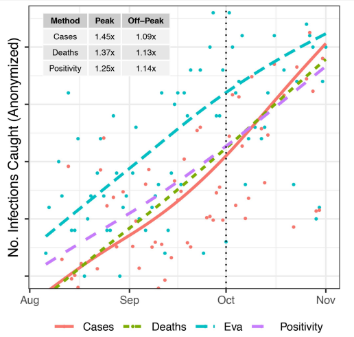
- Using Cases, deaths, positive rates to allocate also underperforms significantly
- Using estimated prevalence probability to grey-list countries prevented 6.7% less infected people from entering
AI Economist
By Harshavardhan Kamarthi
AI Economist
- 332


