Deep Generative models (VAEs) for ODEs with knows and unknowns
Harshavardhan Kamarthi
Data Seminar
Variational Auto-Encoder
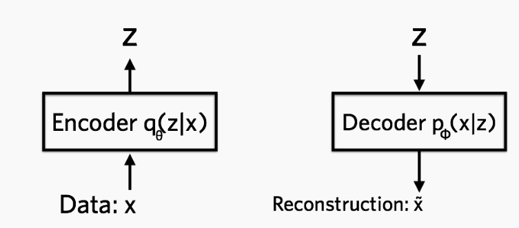
- Goal: Learn distribution p(X)
- Encode x towards a known distribution on latent variable z. Decode z to x
Variational Auto-Encoder

Encoder
Prior on latent variable . Usually set as standard Gaussian.
Decoder
Variational ELBO Loss
Physics based VAEs
- Model data from complex ODEs
- Learn low-dimensional latent representations from data
- Learn relation between observed state and latent state where latent states are governed by ODE
- Learn parameters of the latent ODE
ODE2VAE: Deep generative second order ODEs with Bayesian neural networks

Yidiz et al (NIPS '19)
ODE2VAE: Deep generative second order ODEs with Bayesian neural networks
No information about the functional form
Goals:
- Learn low lank representations from sequential data
- Extrapolate/forecast
Second-order Bayesian ODE

- Second-order: to model higher-order dynamics
- is a Bayesian Neural network with prior
- To capture uncertainty
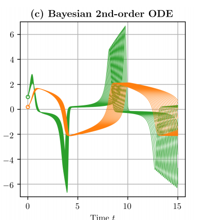
ODE2VAE Model
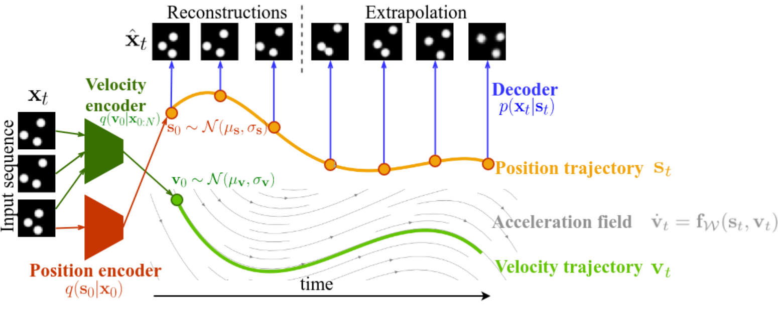
ODE2VAE Encoder

Note:
- Transition function is stochastic
- 3rd equation derived by "Change of variable" theorem (approximated by Runge-Kutta method)
ODE2VAE Decoder

is deterministic NN decoder
ODE2VAE Learning
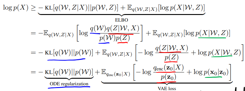

ODE2VAE Learning


- Dynamic loss dominates VAE loss due to long trajectories
- Data may underfit to encoder distribution
- Add regularizer to make ode and encoder distribution similar
Extrapolation Results
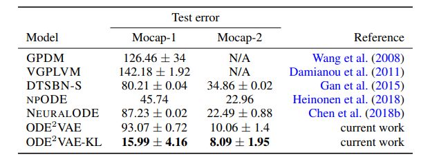
CMU-Walking data (Extrapolate last 1/3 rd trajectory)
Rotating MNIST


Bouncing Ball
Generative ODE Modelling with Known and Unknowns

Linial et al (CHIL '21)
Generative ODE Modelling with Known and Unknowns
Given the functional form:
Estimate
1. Parameters
2. Extrapolate
Encoder
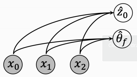
Use RNNs to encode latent variables and then transform to "physics grounded form"
Decoder
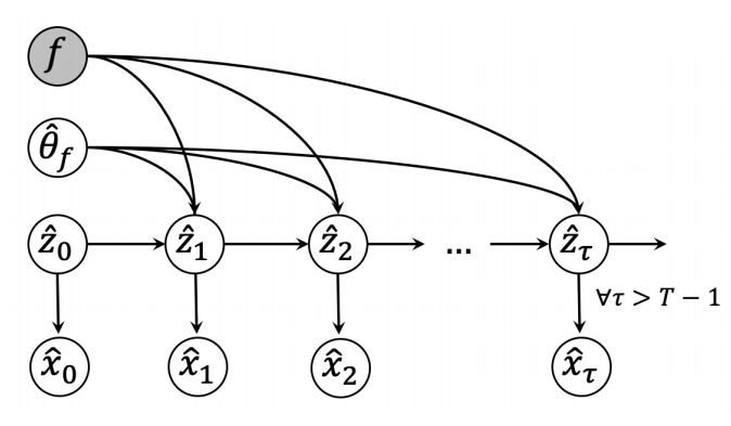
Transition probabilities on latent space is deterministic:
defined from
Transformation to observation space is deterministic via neural network:
defined from
Learning
Generative Distribution
Minimize ELBO
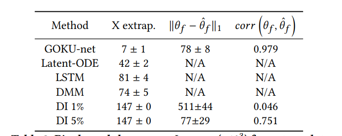
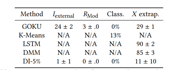
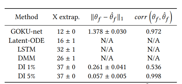
Results
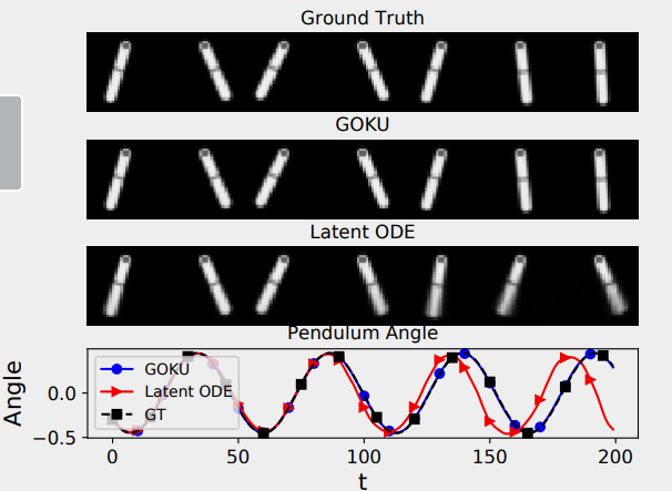
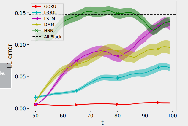
Similarly outperformed baselines significantly for double pendulum a CVS model
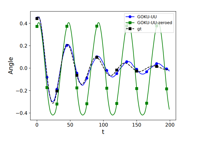
What if part of functional is unknown?
Unknown
Then add NN to learn the unknown:
What if part of functional is unknown?
Physics-Integrated Variational Autoencoders for Robust and Interpretable Generative Modeling
- Functional is partially known

- known part of functional
- Model and extrapolate
Takeishi et al '21
Encoder

- are neural networks, are also trainable parameters

- are defined using domain information
Divide latent encoding into known and unknown parts
Decoder
- is neural network
- is from solution of ODE on
Focusing on Physics-based component
- can dominate training ignoring
- Define a Physics-only reduced model
- Where , the baseline function is another NN with trainable parameter
- Then add regularizer


Physics-based data augmetation
- Goal: ground outputs of which are parameters of
- Idea: Use physics model as data augmentation to train
- Sample from
- Generate
- Train to estimate from
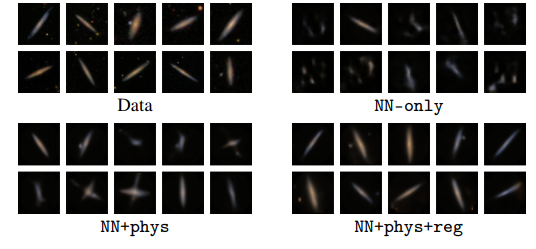
Results

Physice ODE
By Harshavardhan Kamarthi
Physice ODE
- 251


