Benchmarking field-level inference from galaxy surveys

Hugo SIMON-ONFROY,
PhD student supervised by Arnaud DE MATTIA and François LANUSSE
EDSU Tools, 2024/06/07
Benchmarking field-level inference from galaxy surveys

Hugo SIMON-ONFROY,
PhD student supervised by Arnaud DE MATTIA and François LANUSSE
DESI Marseille meeting, 2024/07/12
Field-level inference from galaxy surveys

Hugo SIMON-ONFROY,
PhD student supervised by Arnaud DE MATTIA and François LANUSSE
Rodolphe Clédassou Summer School, 2024/08
The universe recipe (so far)
$$\frac{H}{H_0} = \sqrt{\Omega_r + \Omega_b + \Omega_c+ \Omega_\kappa + \Omega_\Lambda}$$
instantaneous expansion rate
energy content
Cosmological principle + Einstein equation
+ Inflation
\(\delta_L \sim \mathcal G(0, \mathcal P)\)
\(\sigma_8:= \sigma(\delta_L * \Pi_8)\)
initial field
primordial power spectrum
std. of fluctuations smoothed at \(8 \text{ Mpc/h}\)
- Cosmological model links cosmo \(\Omega\) to initial field \(\delta_L\) to galaxy density field \(\delta_g\)
- Cosmological parameter inference obtained via marginalizing full posterior over initial field$$\boldsymbol{p}(\Omega \mid \delta_g) = \int \boldsymbol{p}(\Omega, \delta_L \mid \delta_g) \;\mathrm d \delta_L$$

A high-dimensional inference problem

\(\Omega := \{ \Omega_c, \Omega_b, \Omega_\Lambda, H_0, \sigma_8, n_s,...\}\)


Linear matter spectrum
Structures growth
How to marginalize over such random field?


\(\Omega := \{ \Omega_c, \Omega_b, \Omega_\Lambda, H_0, \sigma_8, n_s,...\}\)
- Find some summary stat \(s\) such that \(\boldsymbol p(\Omega \mid s)\)
- is (more) tractable
- \(\simeq \boldsymbol p(\Omega \mid \delta_g)\) (least information loss)
Use summary statistics

Use summary statistics
Marginalize then sample
- build a marginal model linking cosmo \(\Omega\) and some summary stat \(s\), then simply sample from \(\boldsymbol p(\Omega \mid s)\)
- trade-off analytical/variational tractability vs. info content of \(s\)


summary stat inference
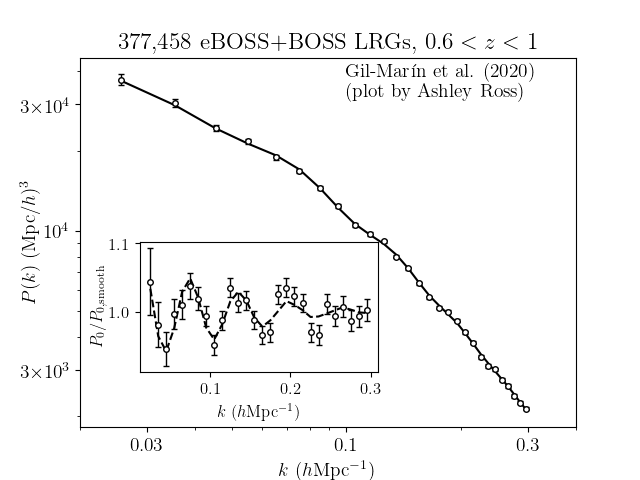
A tractable candidate: the power spectrum
- At large scales, matter density field almost Gaussian so power spectrum is almost lossless compression
- At smaller scales however, matter density field non-Gaussian
Gaussianity and beyond
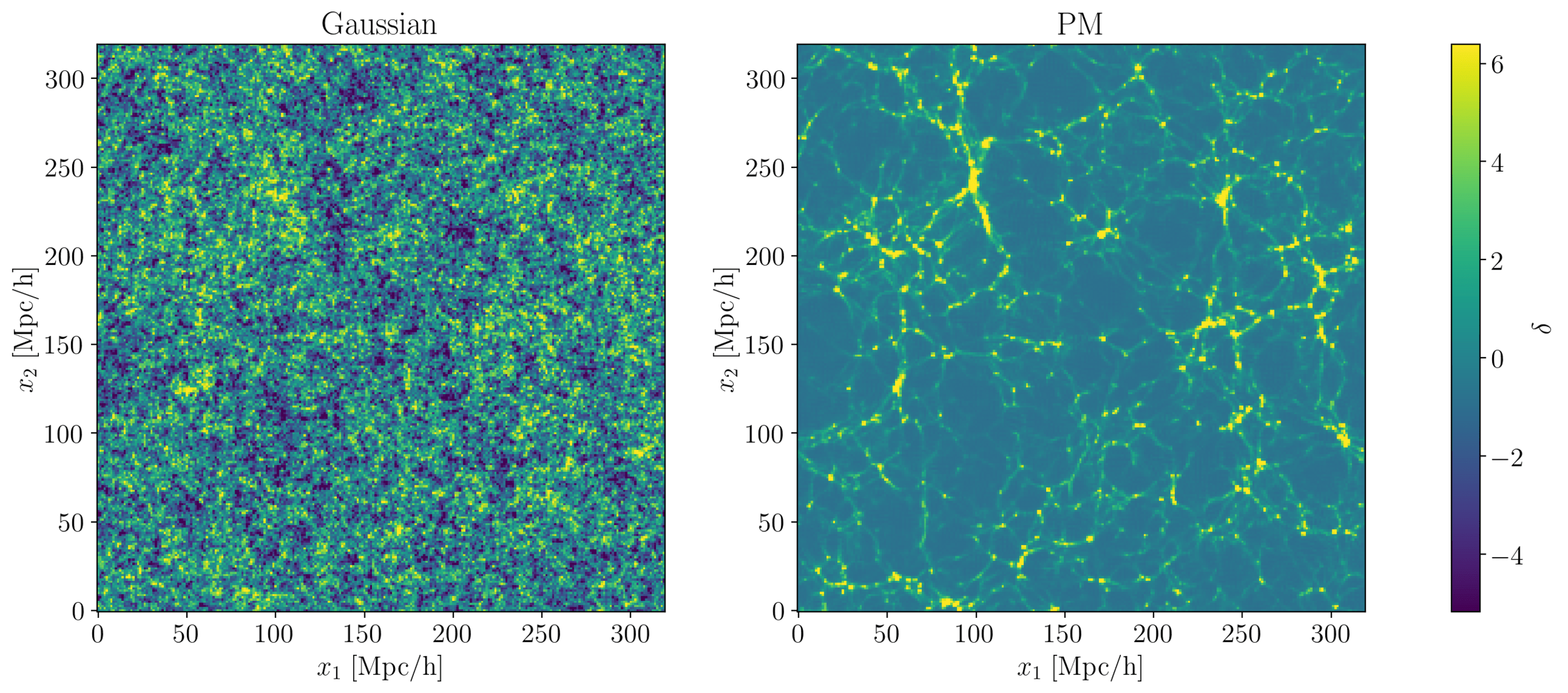
2 fields, same power spectrum: guess which is Gaussian, which is N-body?

Compress or not compress
How much information can we still gain (not lose)?


field-level inference
summary stat inference
Sample then marginalize
- sample jointly \(\Omega\) and \(\delta_L\), then marginalize over \(\delta_L\) samples
- full history reconstruction without info loss
- requires simulating LSS formation for each sample
- For probing non-Gaussian scales of interest in DESI volume \(\operatorname{dim}(\delta_L)\geq1024^3\)

-
Marginalize then sample
- build a marginal model linking cosmo \(\Omega\) and some summary stat \(s\)
- trade-off analytical/variational tractability vs. info content of \(s\)
-
Sample then marginalize
- full history reconstruction without info loss
- requires simulating LSS formation for each sample
Compress or not compress
How much information can we still gain (not lose)?


Model based field-level inference
summary stat inference
We gotta pump this information up
- Field-level
- CNN...
- WST...
- Halo, Peak, Void, Split, Hole...
- 3PCF, Bispectrum
- 2PCF, Power spectrum
- 1D-PDF
$$0-$$
$$\boldsymbol H(\delta_g)-$$


- At large scales, matter density field almost Gaussian so power spectrum is almost lossless compression.
- To prospect smaller non-Gaussian scales, let's use:
Bayes, information flavor

$$\operatorname{\boldsymbol{H}}(X\mid Y) = \boldsymbol{H}(Y \mid X) + \boldsymbol{H}(X) - \boldsymbol{H}(Y)$$
$$= \boldsymbol{H}(X) - \boldsymbol{I}(X;Y) \leq \boldsymbol{H}(X)$$
$$\boldsymbol{H}(X\mid Y_1)$$
$$\boldsymbol{H}(X)$$
$$\boldsymbol{H}( Y_1)$$
$$\boldsymbol{I}(X; Y_1)$$
$$\boldsymbol{H}( Y_2)$$
$$\boldsymbol{I}(X\mid Y_1; Y_2)$$
$$\boldsymbol{H}(X\mid Y_1,Y_2)$$
\(\boldsymbol{H}(X)\) = missing information on \(X\) = amount of bits to communicate \(X\)
The summary stats question in cosmology
$$\boxed{\min_s \operatorname{\boldsymbol{H}}(\Omega\mid s(\delta_g))} = \boldsymbol{H}(\Omega) - \max_s \boldsymbol{I}(\Omega ; s(\delta_g))$$
$$\boldsymbol{H}(\Omega)$$
$$\boldsymbol{H}(\delta_g)$$
$$\boldsymbol{H}(\mathcal s_1)$$
$$\boldsymbol{H}(\mathcal s_2)$$
$$\boldsymbol{H}(\mathcal P)$$
non-Gaussianities
relevant stat
(low info but high mutual info)
irrelevant stat
(high info but low mutual info)
also a relevant stat
(high info and mutual info)
Which stats are relevant for cosmo inference?
More information is better,
but how much better?
Model Based Inference at the field level
(explicitly solve)


Some useful programming tools
-
NumPyro
- Probabilistic Programming Language (PPL)
- Powered by JAX
- Integrated samplers
-
JAX
-
GPU acceleration
- Just-In-Time (JIT) compilation acceleration
- Automatic vectorization/parallelization
- Automatic differentiation
-
GPU acceleration
So JAX in practice?
-
GPU accelerate
- JIT compile
- Vectorize/Parallelize
- Auto-diff
import jax.numpy as np
# then enjoy
function = jax.jit(function)
# function is so fast now!gradient = jax.grad(function)
# too bad if you love chain ruling by handvfunction = jax.vmap(function)
pfunction = jax.pmap(function)
# for-loops are for-loosers


So NumPyro in practice?
def model():
    z = sample('Z', dist.Normal(0, 1))
    x = sample('X', dist.Normal(z**2, 1))
    return x

render_model(model, render_distributions=True)

x_sample = dict(x=seed(model, 42)())
obs_model = condition(model, x_sample)
logp_fn = lambda z: log_density(obs_model,(),{},{'Z':z})[0]
from jax import jit, vmap, grad
score_vfn = jit(vmap(grad(logp_fn)))kernel = infer.NUTS(obs_model)
mcmc = infer.MCMC(kernel, num_warmup, num_samples)
mcmc.run(PRGNKey(43))
samples = mcmc.get_samples()- Probabilistic Programming
- JAX machinery
- Integrated samplers

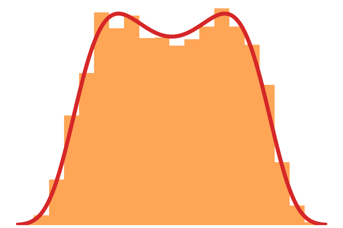

- Prior on
- Cosmology \(\Omega\)
- Initial field \(\delta_L\)
- Dark matter-galaxy connection (Lagrangian galaxy biases) \(b\)
- Initialize matter particles
- LSS formation (LPT+PM)
- Populate matter field with galaxies
- Galaxy peculiar velocities (RSD)
- Observational noise
Now let's build a cosmological model
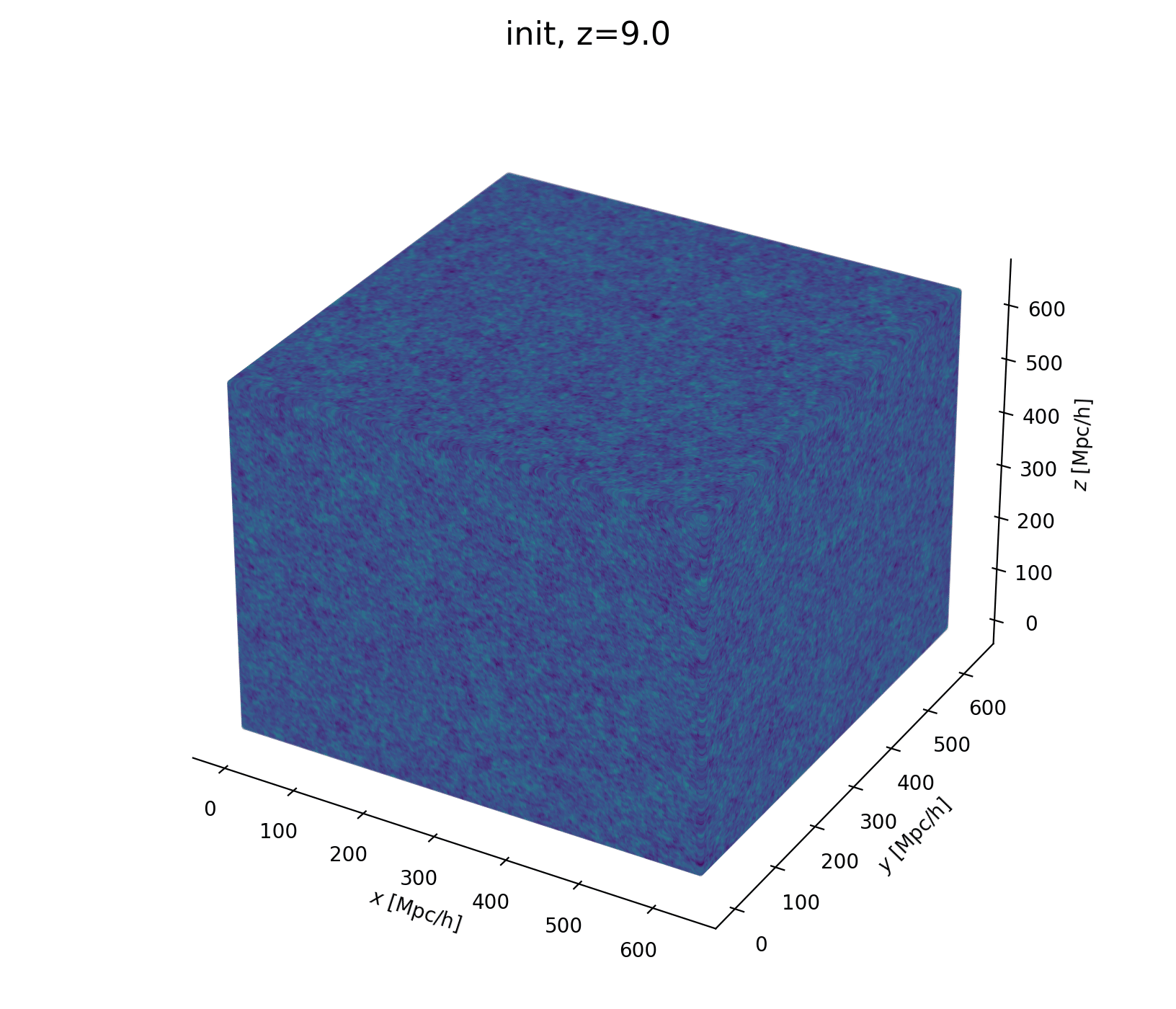
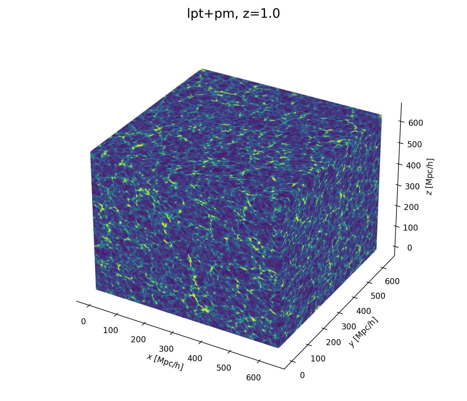


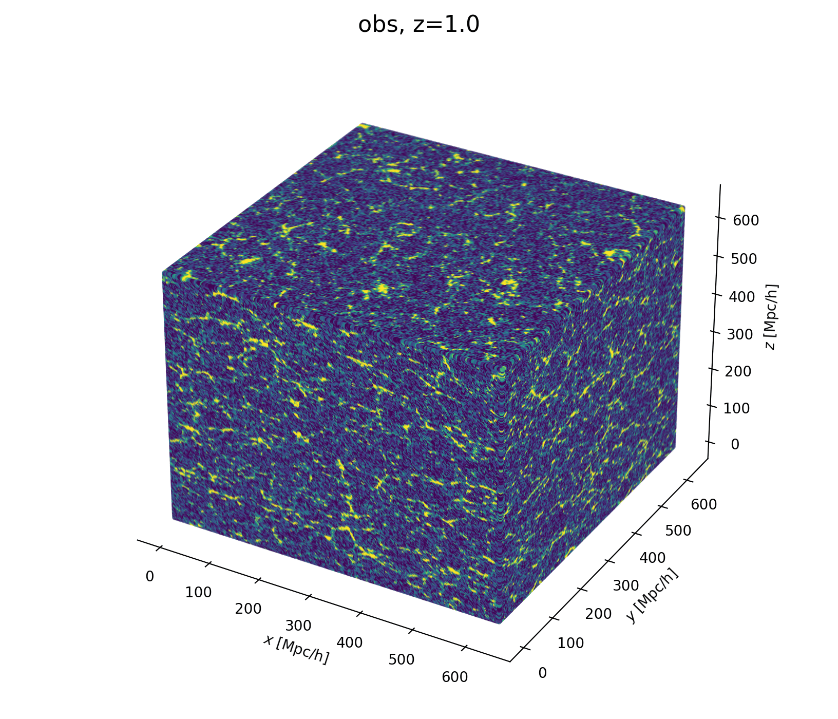
- Fast and differentiable model thx to JaxPM
- still, \(\simeq 1024^3\) parameters is huge!
- Some proposed methods by Lavaux+2018, Bayer+2023
Which sampling methods can scale to high dimensions?

- Prior on
- Cosmology \(\Omega\)
- Initial field \(\delta_L\)
- Dark matter-galaxy connection (Lagrangian galaxy biases) \(b\)
- Cosmology \(\Omega\)
- Initialize matter particles
- LSS formation (LPT+PM)
- Populate matter field with galaxies
- Galaxy peculiar velocities (RSD)
- Observational noise
Now let's build a cosmological model


- \(\simeq 1024^3\) parameters is huge!
- Need inference methods that scale to high dimensions
- Some proposed by Lavaux+2018, Bayer+2023
- Fast and differentiable model
- No need to approx likelihood for your favorite stat from simulation:
the simulation is the likelihood
Why care about differentiable model?
-
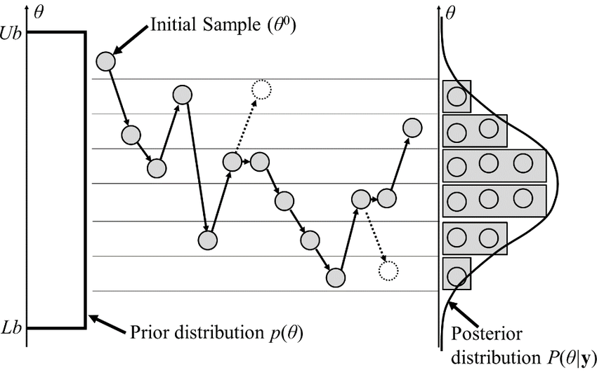
Classical MCMCs
-
agnostic random moves
+ MH acceptance step
= blinded natural selection
- small moves yield correlated samples.
-
agnostic random moves
- SOTA MCMCs rely on the gradient of the model log-proba, to drive dynamic towards highest density regions.

gradient descent
posterior mode
Brownian
exploding Gaussian
Langevin
posterior
+
=


Hamiltonian Monte Carlo (HMC)
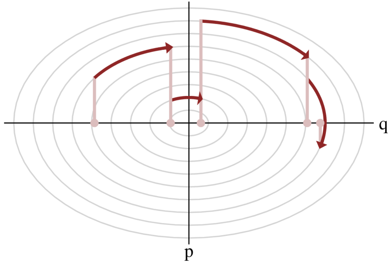
- To travel farther, add inertia.
- sample particle at position \(q\) now have momentum \(p\) and mass matrix \(M\)
- target \(\boldsymbol{p}(q)\) becomes \(\boldsymbol{p}(q , p) := e^{-\mathcal H(q,p)}\), with Hamiltonian $$\mathcal H(q,p) := -\log \boldsymbol{p}(q) + \frac 1 2 p^\top M^{-1} p$$
- at each step, resample momentum \(p \sim \mathcal N(0,M)\)
- let \((q,p)\) follow the Hamiltonian dynamic during time length \(L\), then arrival becomes new MH proposal.

Variations around HMC
-
No U-Turn Sampler (NUTS)
- trajectory length \(L\) auto-tuned
- samples drawn along trajectory
- NUTSGibbs i.e. alternating sampling over parameter subsets.
Why care about differentiable model?

Variations around HMC
-
No U-Turn Sampler (NUTS)
- trajectory length auto-tuned
- samples drawn along trajectory
- NUTSGibbs i.e. alternating sampling over parameter subsets
-
Model gradient drives sample particles towards higher density regions
-
Hamiltonian Monte Carlo (HMC):
to travel farther, add inertia
- Yields less correlated chains

3) Hamiltonian dynamic
1) mass \(M\) particle at \(q\)
2) random kick \(p\)
2)random kick \(p\)
1) mass \(M\) particle at \(q\)
3) Hamiltonian dynamic
-
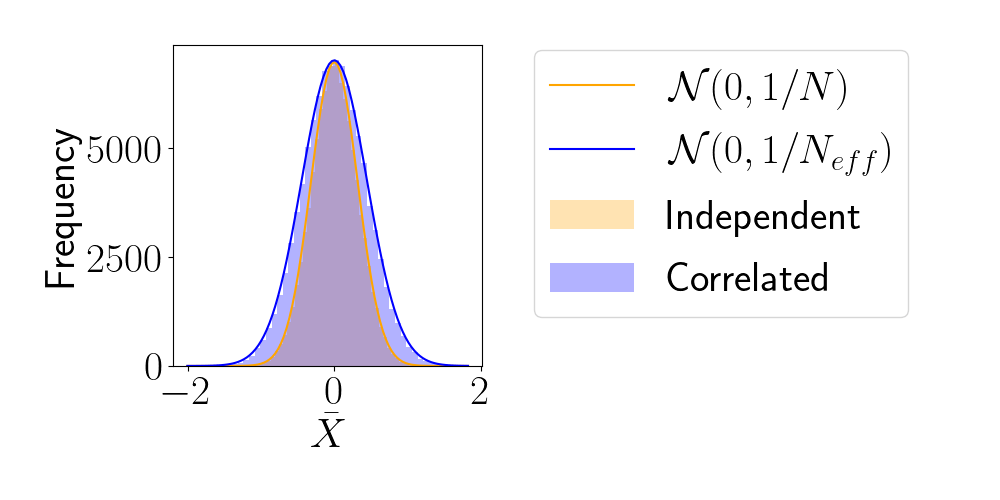
Effective Sample Size (ESS)
- number of i.i.d. samples that yield same statistical power.
- For sample sequence of size \(N\) and autocorrelation \(\rho\) $$N_\textrm{eff} = \frac{N}{1+2 \sum_{t=1}^{+\infty}\rho_t}$$so aim for as less correlated sample as possible.
- Main limiting computational factor is model evaluation (e.g. N-body), so characterize MCMC efficiency by \(N_\text{eval} / N_\text{eff}\)
How to compare samplers?

Benchmarking
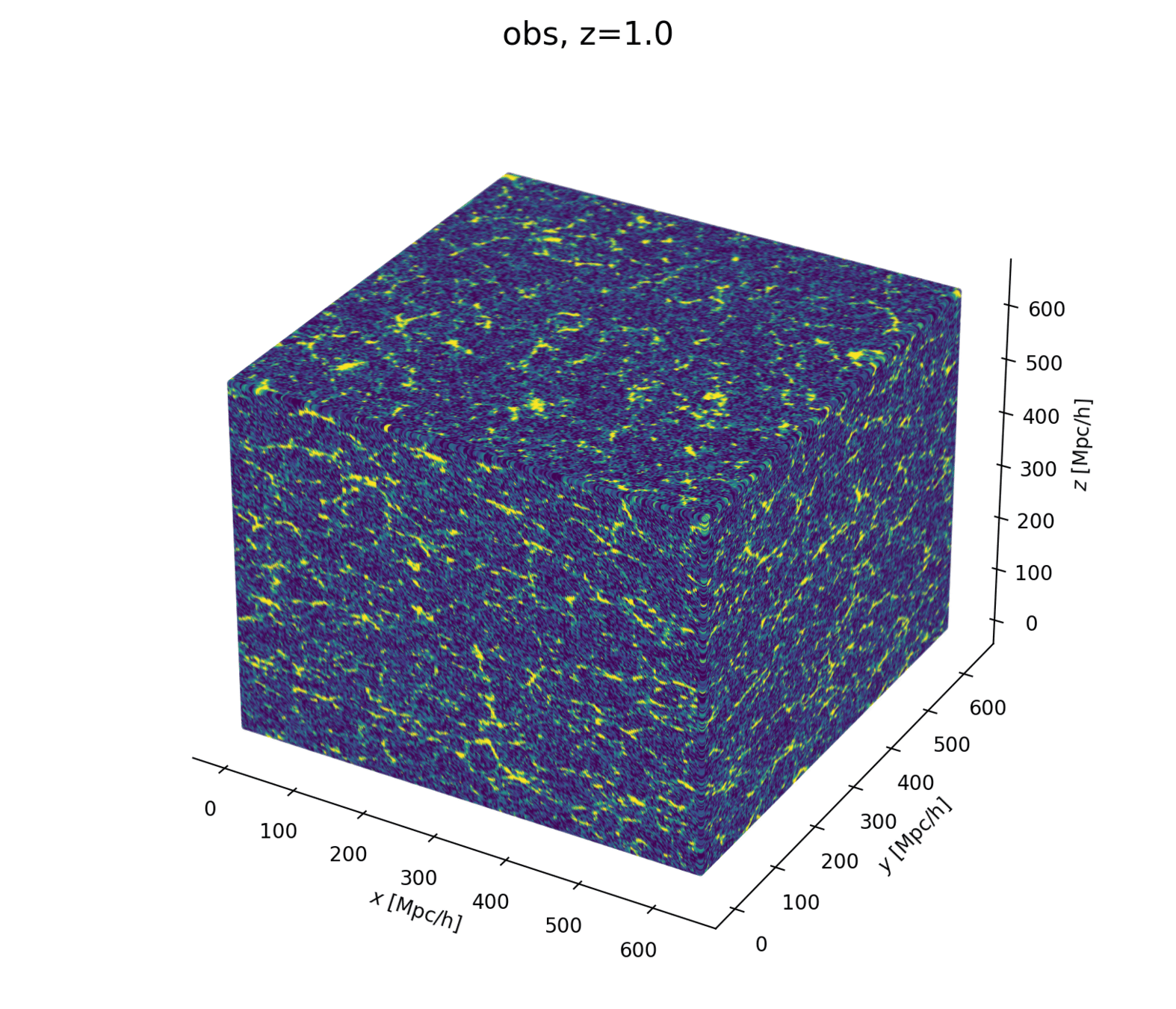
- model setting: \(64^3\) mesh, \((640\textrm{ Mpc/h})^3\) box, 1LPT, 2nd order Lagrangian bias expansion, RSD and Gaussian observational noise.
- parameter space: initial field \(\delta_L\), cosmology \(\Omega\! =\! \{\Omega_m, \sigma_8\}\), and galaxy biases \(b\!=\!\{b_1,b_2,b_{s^2},b_{\nabla^2}\}\). Total of \(64^3 + 2 +4\) parameters.
- For NUTSGibbs: split sampling between \(\delta_L\) and the rest (common in lit.)
- Results suggest no particular advantage to splitting sampling between initial field and rest.


Reconstruct the initial field simultaneously, yielding posterior on full universe history
number of evaluations to yield one effective sample: the higher the worse
Large scale field-level inference
prelim
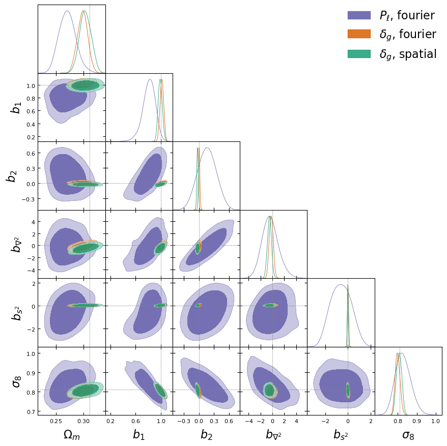
- High-dimensional sampling based on Hamiltonian Monte Carlo (HMC)
-
Model gradient drives sample particles towards high density regions
- Yields less correlated chains

Infer cosmo and initial field jointly, yielding posterior over full universe history
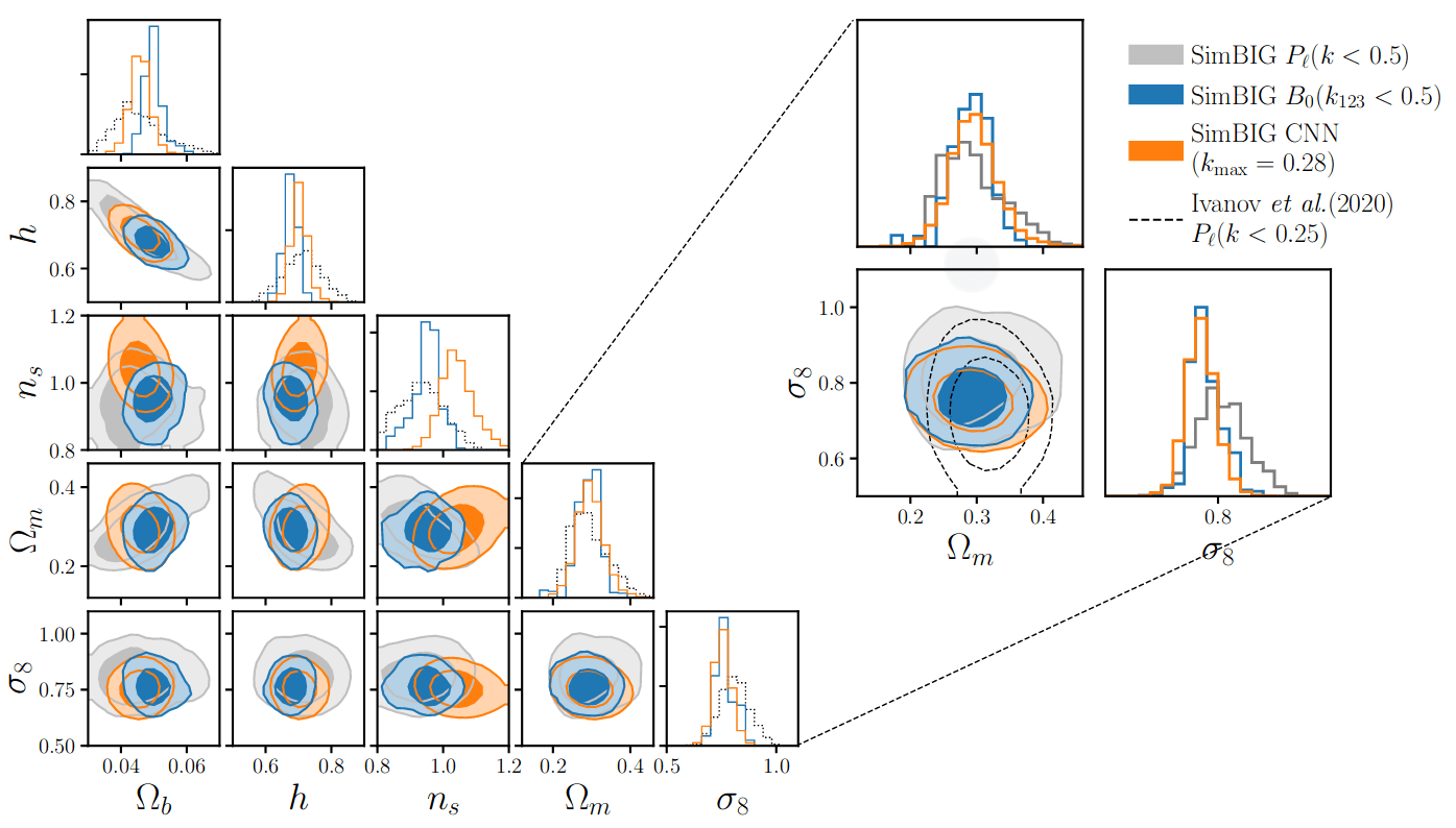
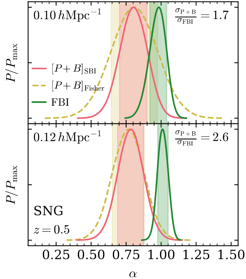
Information content comparison
...and what's next
- Benchmark more proposed samplers.
- Compare to SBI approaches.
- Move towards applications on DESI.
Recap...
-
Leverage modern computational tools to build fast and differentiable cosmological model.
-
Field-level inference can scale to Stage-IV galaxy surveys, and may be relevant to fully capture cosmological information from data.

...and what's next
- Include more proposed samplers.
- Compare to SBI approaches.
- Move towards applications on DESI data.
Recap...
-
Field-level inference may be relevant to fully capture cosmological information in data.
-
Leverage modern computational tools to build fast and differentiable cosmological model.
-
Standardized benchmark for comparing MCMC samplers on field-level inference tasks, selecting proposed methods for Stage-IV galaxy surveys.
2024EDSU
By hsimonfroy
2024EDSU
- 17
