Implicit full-field inference for LSST weak Lensing
Justine Zeghal
Supervisors: François Lanusse, Alexandre Boucaud, Eric Aubourg
Tri-state Cosmology x machine learning journal club
January 19, Paris, France



Cosmological context
Cosmological context
Cosmological context
Cosmological context
How to extract all the information embedded in our data?
Standard analysis relies on 2-point statistics and use a Gaussian analytic likelihood.
But these summary statistics is suboptimal at small scales..
Full-field inference 2 ways..
- Bayesian hierarchical modeling
Full-field inference 2 ways..
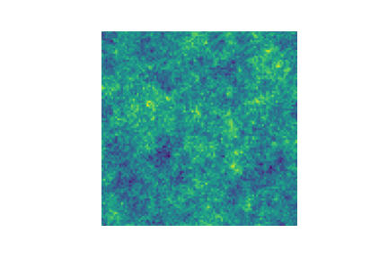
Full-field inference 2 ways..
- Bayesian hierarchical modeling
Explicit joint likelihood
Full-field inference 2 ways..
- Bayesian hierarchical modeling

And then run an MCMC to get the posterior:
And then run an MCMC to get the posterior:
- Bayesian hierarchical modeling
Explicit joint likelihood
Full-field inference 2 ways..

It provides exact results but necessitates the BHM to be differentiable and requires a lot of simulations.
And then run an MCMC to get the posterior:
And then run an MCMC to get the posterior:
- Bayesian hierarchical modeling
Explicit joint likelihood
Full-field inference 2 ways..

- Implicit inference with sufficient statistics
Full-field inference 2 ways..
- Implicit inference with sufficient statistics
Full-field inference 2 ways..

- Implicit inference with sufficient statistics
Full-field inference 2 ways..
Simulator

Summary statistics
- Implicit inference with sufficient statistics
Full-field inference 2 ways..
Simulator

- Implicit inference with sufficient statistics
Full-field inference 2 ways..
Simulator
And use neural-based likelihood-free approaches to get the posterior
using only:
Summary statistics

And use neural-based likelihood-free approaches to get the posterior
using only:
- Implicit inference with sufficient statistics
Full-field inference 2 ways..
Simulator
Summary statistics

And use neural-based likelihood-free approaches to get the posterior
using only:
- Implicit inference with sufficient statistics
Full-field inference 2 ways..
Simulator
Summary statistics

And use neural-based likelihood-free approaches to get the posterior
using only:
- Implicit inference with sufficient statistics
Full-field inference 2 ways..
Simulator
Summary statistics

Simulator
Summary statistics

Outline
Simulator
Summary statistics

1. Focus on optimal compression
Outline
Simulator
Summary statistics

1. Focus on optimal compression
2. Focus on optimal and simulation-efficient inference
Outline
Optimal Neural Summarisation for Full-Field Cosmological Implicit Inference
Denise Lanzieri, Justine Zeghal
T. Lucas Makinen, Alexandre Boucaud, François Lanusse, and Jean-Luc Starck


How to extract all the information?
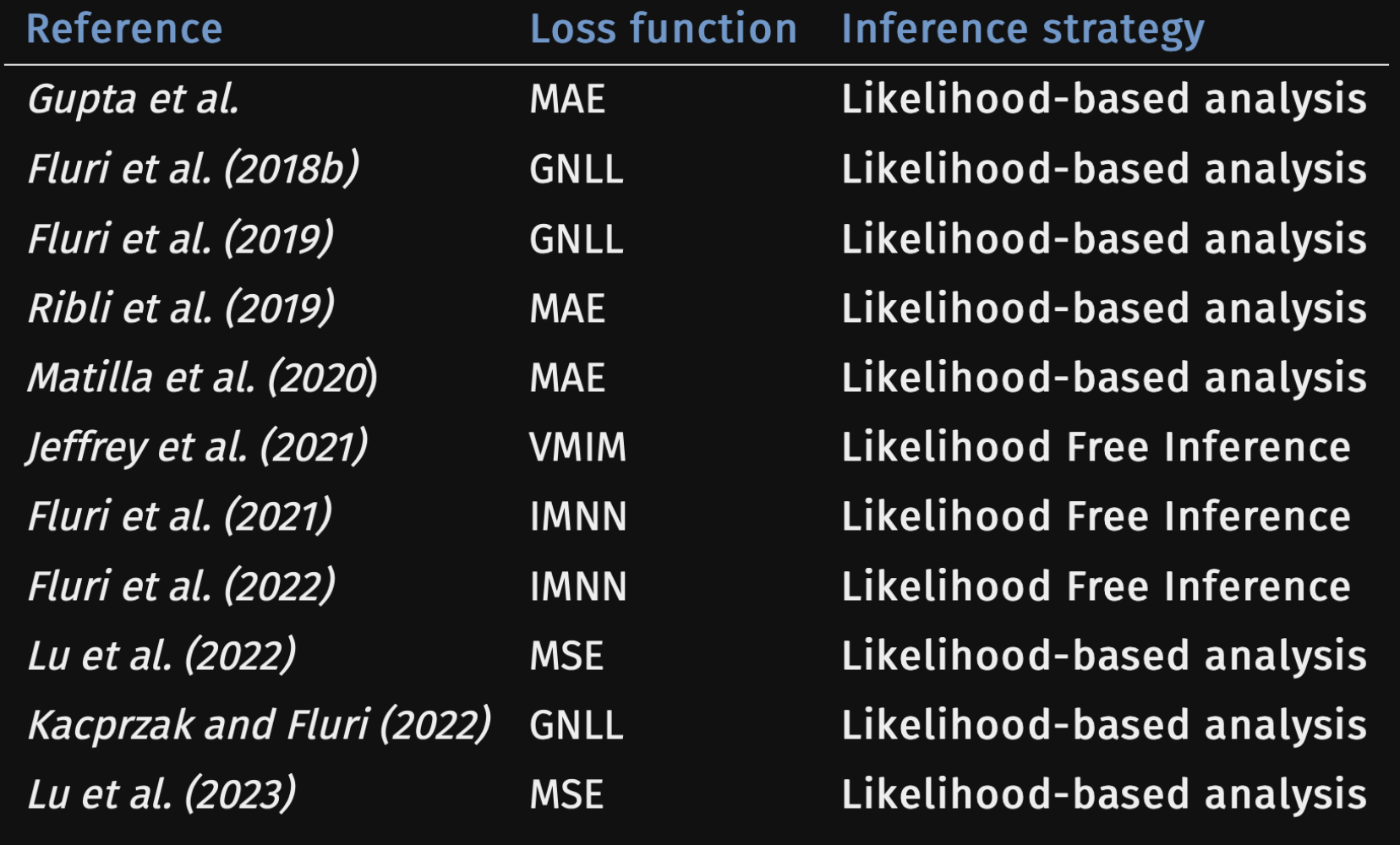
It is only a matter of the loss function you use to train your compressor..

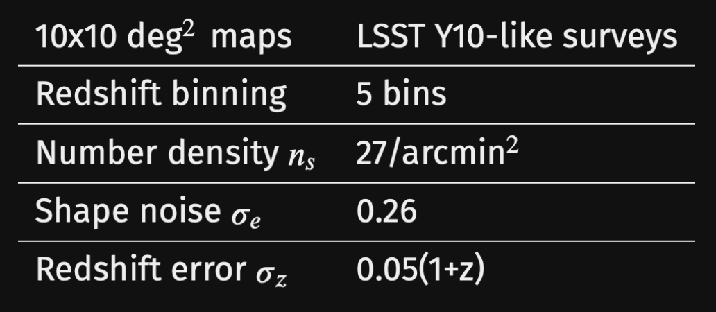
We developed a fast and differentiable (JAX) log-normal mass maps simulator
For our benchmark: a Differentiable Mass Maps Simulator

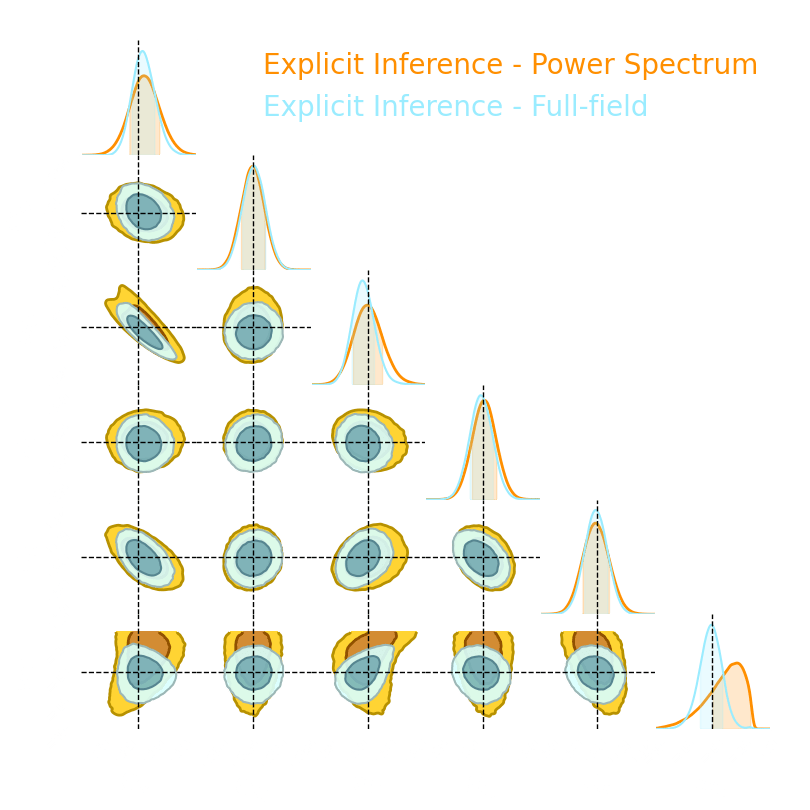
Numerical results
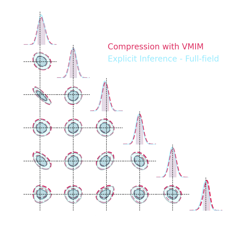
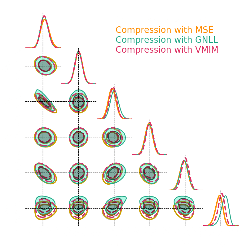
1. We compress using one of the 5 losses.
Benchmark procedure:
2. We compare their extraction power by comparing their posteriors.
For this, we use a neural-based likelihood-free approach, which is fixed for all the compression strategies.
Simulator
Summary statistics

1. Focus on optimal compression
2. Focus on optimal and simulation-efficient inference
Outline
Simulation-Efficient Implicit Inference.
Is differentiability useful?
Justine Zeghal
Denise Lanzieri, Alexandre Boucaud, François Lanusse, and Eric Aubourg
-
do gradients help implicit inference methods?
In the case of weak lensing analysis,
-
which inference method requires the fewest simulations?
Log-normal LSST Y10 like
differentiable
simulator

For our benchmark

-
do gradients help implicit inference methods?


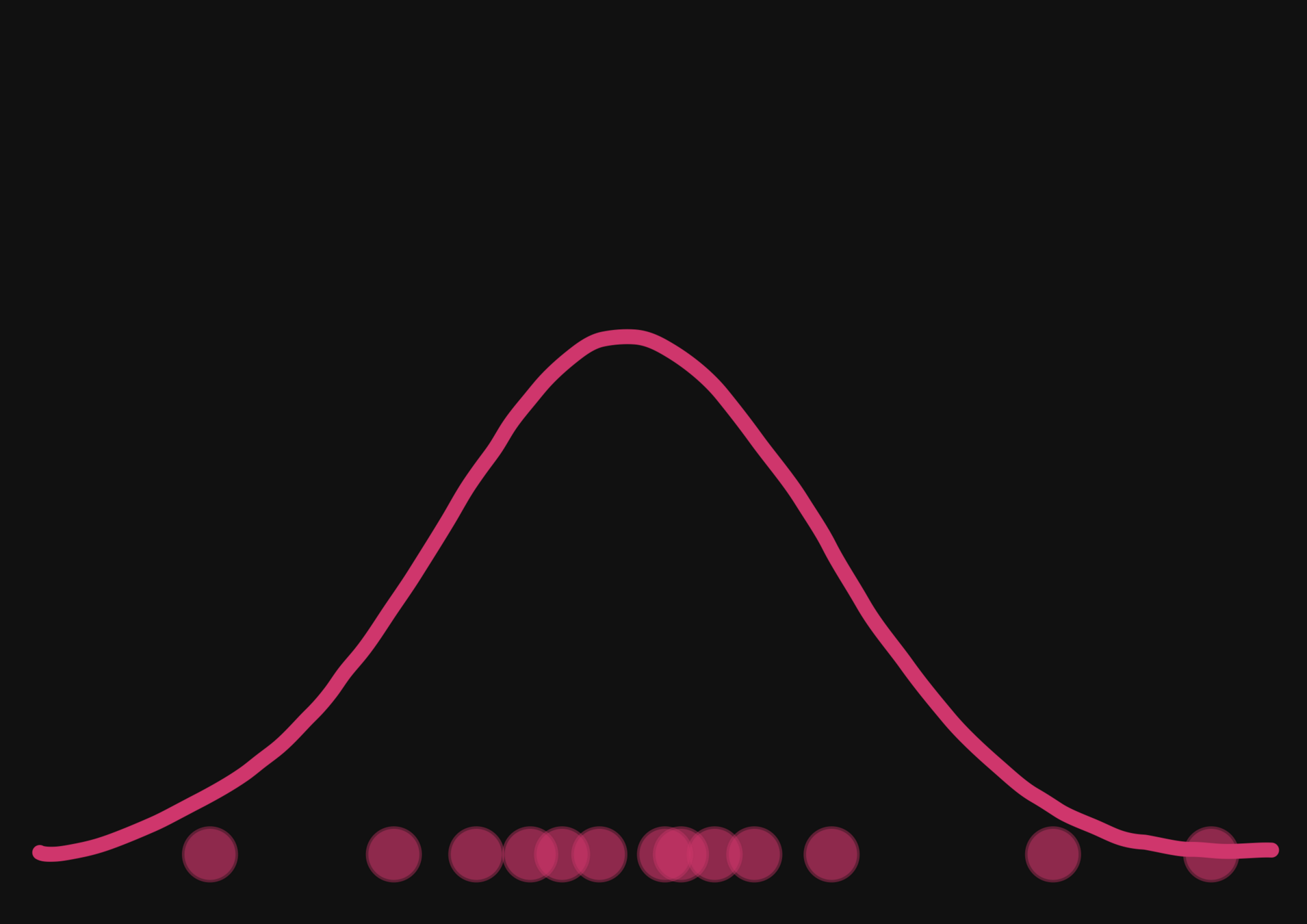

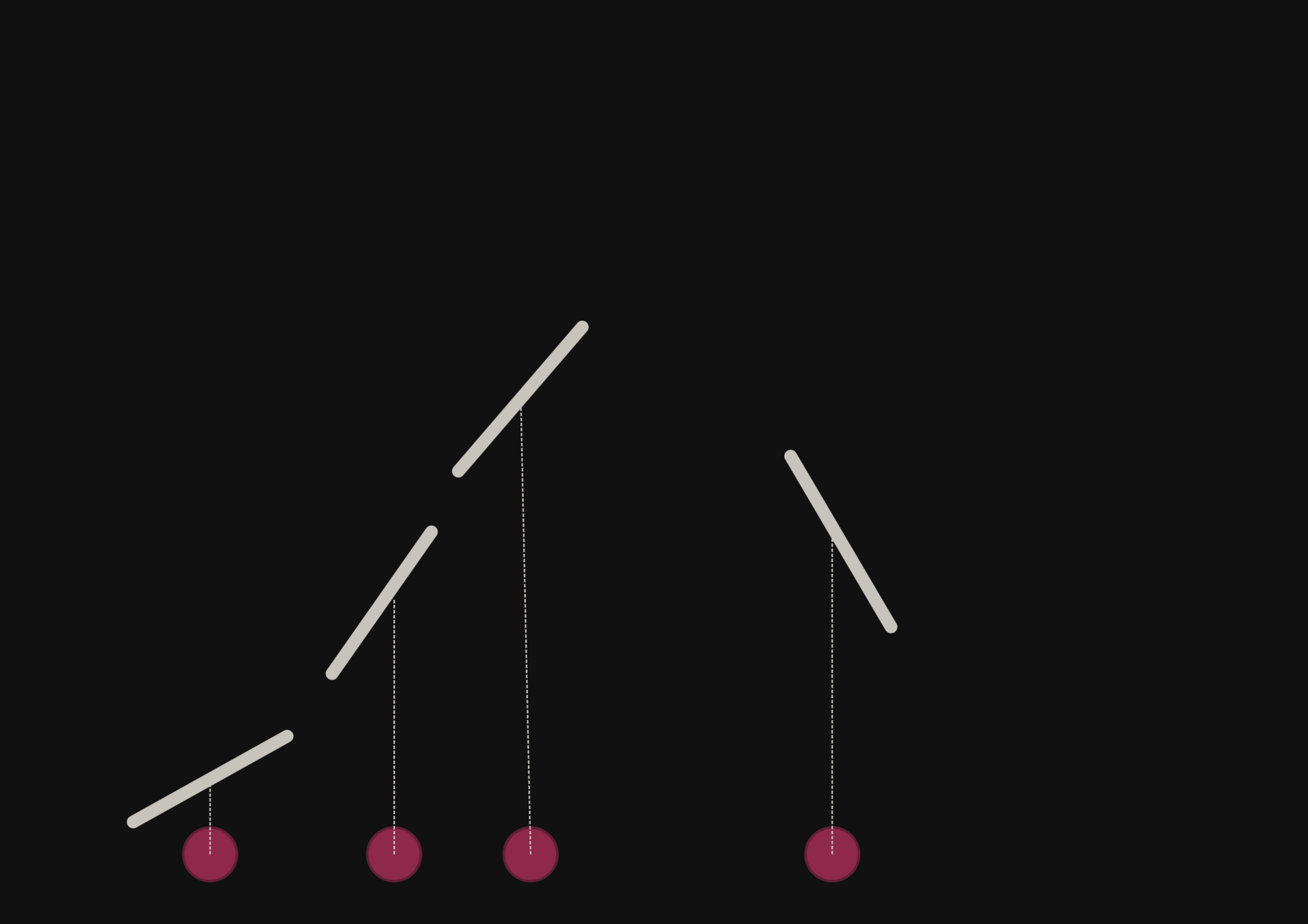
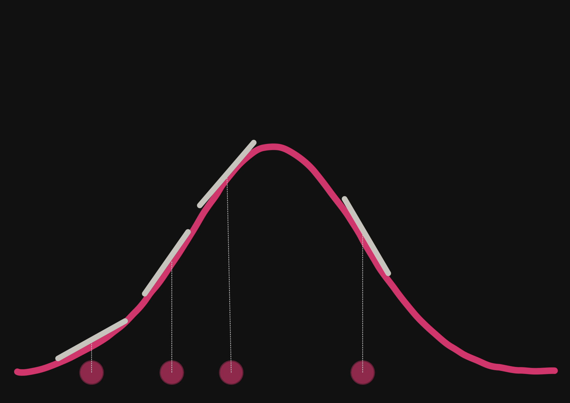
With a few simulations it's hard to approximate the posterior distribution.
→ we need more simulations
BUT if we have a few simulations
and the gradients
(also know as the score)
then it's possible to have an idea of the shape of the distribution.
-
do gradients help implicit inference methods?
Normalizing flows are trained by minimizing the negative log likelihood:
-
do gradients help implicit inference methods?
Normalizing flows are trained by minimizing the negative log likelihood:
-
do gradients help implicit inference methods?
But to train the NF, we want to use both simulations and gradients
Normalizing flows are trained by minimizing the negative log likelihood:
-
do gradients help implicit inference methods?
But to train the NF, we want to use both simulations and gradients
Normalizing flows are trained by minimizing the negative log likelihood:
-
do gradients help implicit inference methods?
But to train the NF, we want to use both simulations and gradients
Normalizing flows are trained by minimizing the negative log likelihood:
-
do gradients help implicit inference methods?
Problem: the gradient of current NFs lack expressivity
But to train the NF, we want to use both simulations and gradients
Normalizing flows are trained by minimizing the negative log likelihood:
-
do gradients help implicit inference methods?
Problem: the gradient of current NFs lack expressivity
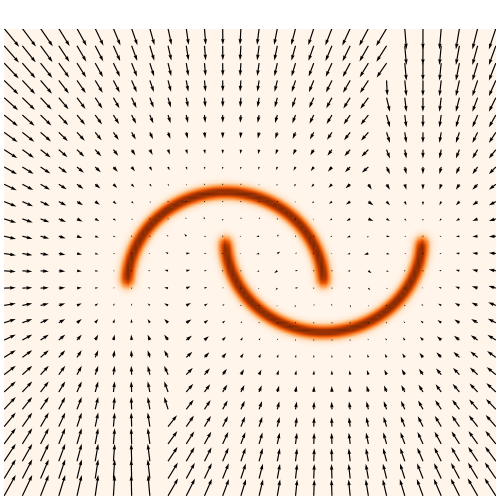
But to train the NF, we want to use both simulations and gradients
Normalizing flows are trained by minimizing the negative log likelihood:
-
do gradients help implicit inference methods?
Problem: the gradient of current NFs lack expressivity
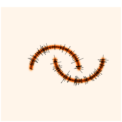
But to train the NF, we want to use both simulations and gradients
Normalizing flows are trained by minimizing the negative log likelihood:
-
do gradients help implicit inference methods?
Problem: the gradient of current NFs lack expressivity

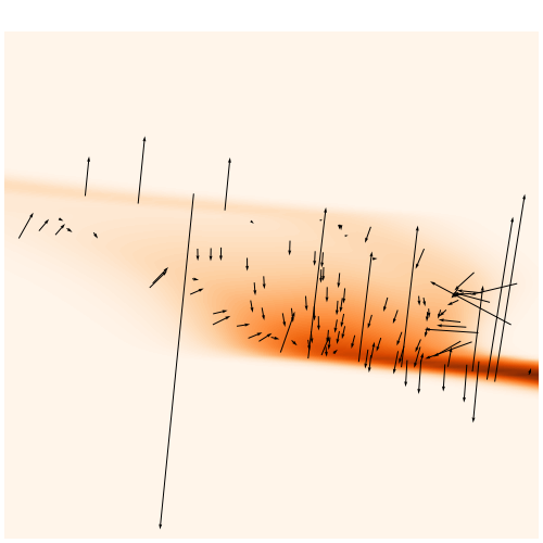
But to train the NF, we want to use both simulations and gradients
Normalizing flows are trained by minimizing the negative log likelihood:
-
do gradients help implicit inference methods?
Problem: the gradient of current NFs lack expressivity


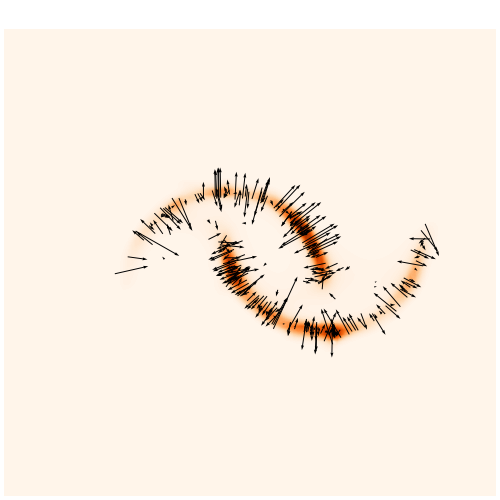
But to train the NF, we want to use both simulations and gradients


→ On our toy Lotka Volterra model, the gradients helps to constrain the distribution shape

-
do gradients help implicit inference methods?
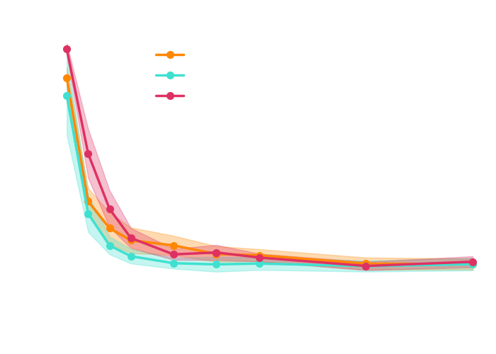
(from the simulator)
(requires a lot of additional simulations)
→For this particular problem, the gradients from the simulator are too noisy to help.
-
do gradients help implicit inference methods? ~ LSST Weak Lensing case
-
do gradients help implicit inference methods?
In the case of weak lensing analysis,
-
which inference method requires the fewest simulations?
Log-normal LSST Y10 like
differentiable
simulator

For our benchmark

-
which inference method requires the fewest simulation?

Focus on implicit inference methods
-
which inference method requires the fewest simulation?
simulations
simulations
more than
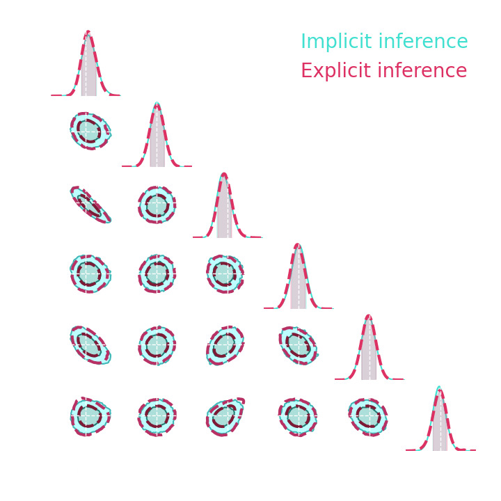
Simulator
Summary statistics

Thank your for your attention!
contact: zeghal@apc.in2p3.frslides at: https://slides.com/justinezgh
Copy of Tri-state Cosmology x machine learning journal club
By hsimonfroy
Copy of Tri-state Cosmology x machine learning journal club
- 257


