Hugo Hadfield
Cambridge University PhD student, Signal Processing and Communications Laboratory
If \(T_i^2 < 0\) then the point is unreachable
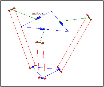
- Move only one motor
- This fixes two of the spheres, they intersect in a circle
- We are therefore interested in the differential of the end point of the point pair made from intersection of the circle and the moving sphere
- First we need to find how the center of the sphere changes as we move theta
- How does point pair move with the sphere?
- Now we need to know how the conformal endpoint of the point pair changes
- How does the 3D endpoint change with the conformal endpoint change? (derivative of 'down' function)
- We now have a closed form expression for the derivative of the endpoint wrt. theta and we didn't have to use maple once!
- We can use this for control and optimisation. Consider a cost function:
- We therefore have a closed form for
and so can do gradient descent
- Given the forward jacobian we can simply invert the 3x3 matrix at each point to get the inverse jacobian
OR
- We can differentiate our inverse kinematic equations..
Starting with Sigma_i
Differentiate wrt. a scalar param \alpha
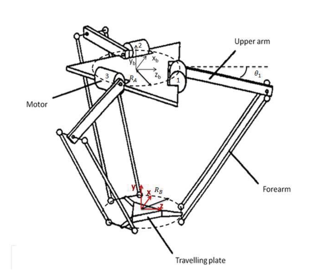
the sphere centred at the meeting of the 4 bar mechanism and the end platform
- Now we need to know how the elbow positions vary with \alpha
- Here A_i is the conformal elbow position
- Finally we need to know how the joints vary with elbow position
- We are done (Once again no Maple!)
- The inverse jacobian allows us to map velocity of the endpoint to velocity of joints
- In other words, to minimise cost at maximum rate drive the end point linearly at our target point (obviously)
- With the inverse jacobian we can do exactly that
- CGA provides a very neat framework for solving the forward and inverse kinematics of parallel robots
- We can easily simulate the dynamics of the robot with clifford and ganja.js
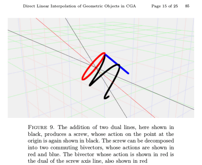
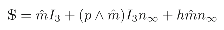
- Trivectors in CGA represent lines and circles
- The direct interpolation of lines and circles results in trivectors interpretable as general screws
- Screw theory is widely used in robotics for analysis of kinematics and dynamics
- Lets bring screw theory and CGA (also PGA) together properly and analyse a whole load of systems
By Hugo Hadfield
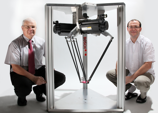
The delta robot is one of the most popular parallel robots that exist, known for its speed and precision. This presentation covers the forward and inverse kinematics of the delta robot using Conformal Geometric Algebra. This material makes up a part of my PhD thesis here https://hh409.user.srcf.net/thesis/thesis.html


