Intro to GA for CS

Hugo Hadfield

June 2020

Geometric/Clifford Algebra

  • GA is about studying the properties of the real Clifford algebras
  • We typically describe which algebra we are working in with the following syntax:
Cl(p, q, r)
  • This syntax defines a set of basis vectors
  • For these basis vectors we define the geometric product:
e_ie_i = 1
e_ie_i = -1
e_ie_i = 0

p vectors

q vectors

r vectors

  • For vectors this product is anticommutative:
e_ie_j = -e_je_i

Example 3D GA

Cl(3, 0, 0)
  • Consider the algebra:
  • This creates 3 basis vectors that square to 1:
e_1e_1 = 1, \, e_2e_2 = 1, \, e_3e_3 = 1
e_1e_2 = -e_2e_1 = e_{12}
  • We will write the product of two vectors with the shorthand:
(e_1 + e_2)(e_1 + e_3) = e_1e_1 + e_2e_1 + e_2e_3 + e_1e_3 \\ = 1 - e_{12} + e_{23} + e_{13}
  • The geometric product is distributive and associative:
e_{123}e_1 = e_1e_2e_3e_1 = -e_2e_1e_3e_1 = e_2e_3e_1e_1 = e_2e_3

Grade Selection

(e_1 + e_2)(e_1 + e_3) = 1 - e_{12} + e_{23} + e_{13}
  • Define another operation, the grade selection operation:
\left< 1 - e_{12} + e_{23} + e_{13}\right>_0 = 1
\left< 1 - e_{12} + e_{23} + e_{13}\right>_2 = - e_{12} + e_{23} + e_{13}
  • If there is nothing of the grade in there, then it gives 0:
\left< 1 - e_{12} + e_{23} + e_{13}\right>_1 = 0
  • Consider the result:
(e_1 + e_2)(e_1 + e_3) = \left< (e_1 + e_2)(e_1 + e_3) \right>_0 + \left< (e_1 + e_2)(e_1 + e_3) \right>_2\\ = 1 - e_{12} + e_{23} + e_{13}
  • The result of the geometric product can be written with grade selection:

Inner and Outer Products

  • Consider the result:
(e_1 + e_2)(e_1 + e_3) = \left< (e_1 + e_2)(e_1 + e_3) \right>_0 + \left< (e_1 + e_2)(e_1 + e_3) \right>_2\\ = 1 - e_{12} + e_{23} + e_{13}

Inner (dot) product

  • This motivates us to define two new products:

Outer (wedge) product

X_a\wedge Y_b = \left< X_a Y_b \right>_{a+b}
X_a\cdot Y_b = \left< X_a Y_b \right>_{|a-b|}
  • For vectors in GA this leads us to the result:
ab = a \cdot b + a \wedge b

What is it good for?

  • Each algebra can be viewed as a domain specific language for some specific geometry
  • All the algebras share the same basic operations, learn them once, use them everywhere
  • Cl(3,0,0)  - 3D vectors, quaternions, projections
  • Cl(4,0,0)  - Homogeneous points, lines, planes, rotations, projections
  • Cl(3,0,1)  - Homogeneous points, lines, planes, projections, intersections, dual quaternions, screw theory, rigid body dynamics
  • Cl(4,1,0)  - Everything in Cl(3,0,1) + line-segments, circles, spheres, all conformal transformations, distance geometry
  • Cl(4,2,0)  - 3D Lie Sphere Geometry
  • Cl(4,4,0)  - Homogeneous points, lines, quadrics, rotations, shear transformations
  • Cl(8,2,0)  - Everything in Cl(4,1,0) + Quadrics, Dupin Cyclides + probably a lot more

Algebras for 3D Euclidean space (there are lots more):

Some algebras for non-Euclidean space (there are lots more):

  • Cl(1,3,0)  - Space time algebra, Lorentz transformations, electromagentism
  • Cl(4,0,0)  - Spherical and hyperbolic space, quantum mechanics

Serial Robot Forward Kinematics CGA

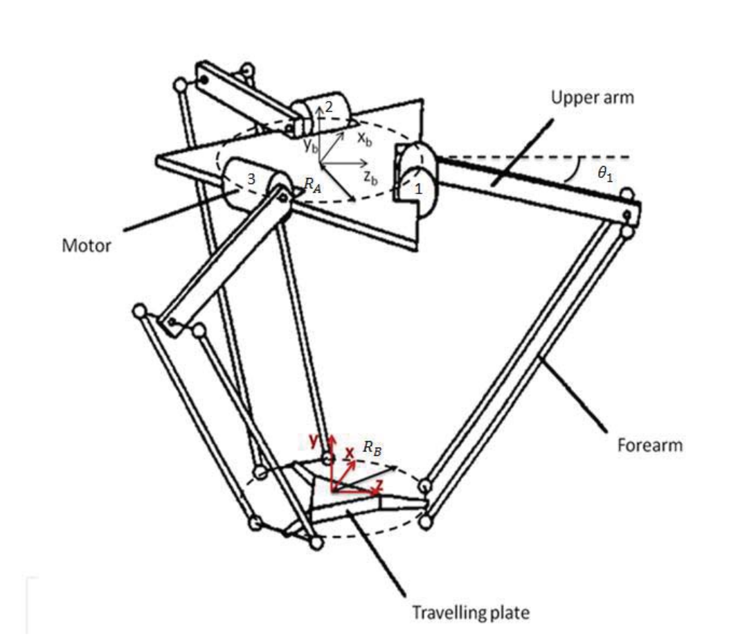
Can we construct a rotor from origin to endpoint?

R_0 = \cos(\theta_0/2) + \sin(\theta_0/2)e_1\wedge e_3
R_1 = \cos(\theta_1/2) + \sin(\theta_1/2)e_1\wedge e_2
\newcommand{\la}{\langle} \newcommand{\ra}{\rangle} \newcommand{\nn}{\nonumber} \newcommand{\ninf}{n_{\infty}} \newcommand{\einf}{e_{\infty}} \newcommand{\no}{n_{0}} \newcommand{\eo}{e_{0}} \newcommand{\wdg}{\wedge} \newcommand{\pdiff}[2]{\frac{\partial #1}{\partial #2} } R_\rho = 1 - \frac{1}{2}\rho e_1\wedge \ninf
R_2 = \cos(\theta_2/2) + \sin(\theta_2/2)e_1\wedge e_2
\newcommand{\la}{\langle} \newcommand{\ra}{\rangle} \newcommand{\nn}{\nonumber} \newcommand{\ninf}{n_{\infty}} \newcommand{\einf}{e_{\infty}} \newcommand{\no}{n_{0}} \newcommand{\eo}{e_{0}} \newcommand{\wdg}{\wedge} \newcommand{\pdiff}[2]{\frac{\partial #1}{\partial #2} } R_l = 1 + \frac{1}{2}l e_1\wedge \ninf
R = R_0R_1R_\rho R_2R_l
\newcommand{\no}{n_{0}} Y = R\no\tilde{R}

Construct the base rotors

Construct the first link's translation rotor

Construct the elbow and link 2 translation rotor

The combined rotor is the product of all of them

\rho
l
y
\theta_0
\theta_1
\theta_2
x

Serial Robot Inverse Kinematics

\rho
l
y
\theta_0
\theta_1
\theta_2
\newcommand{\ninf}{n_{\infty}} S_Y = I_5(Y - \frac{1}{2}l^2\ninf)
\newcommand{\ninf}{n_{\infty}} S_{\text{base}} = I_5(n_0 - \frac{1}{2}\rho^2\ninf)
C = S_Y\vee S_{\text{base}}
\newcommand{\ninf}{n_{\infty}} \Pi = n_0\wedge up(e_3)\wedge Y\wedge \ninf
\newcommand{\ninf}{n_{\infty}} P = \Pi\vee C
\newcommand{\ninf}{n_{\infty}} X = \left[1 + \frac{P}{\sqrt{P\tilde{P}}}\right](P\cdot\ninf)
x

(If \(P^2 < 0 \) then y is out of reach)

Construct a sphere at the base, \(n_0\)

Construct a sphere at the endpoint, y

Intersect the spheres to give a circle

Define a vertical plane through the endpoint and base

Intersect the circle and the plane to give a point pair

Choose one of the elbow position solutions

x = -\frac{-\sum_{j=1}^{j=3}(X\cdot e_j)e_j}{X\cdot n_\infty}

\( A \vee B \) is just \( I_5(I_5A \wedge I_5B) \)

\( I_5 = e_1e_2e_3e_4e_5 \)

Model of a Delta Robot

Forward Kinematics

a_i = (r_b - r_e + l\cos(\theta_i))s_i + l\sin(\theta_i)e_3

Get the pseudo-elbow point \(A_i\)

Y = -\tilde{P}(T\cdot n_\infty)P\\ y = \frac{-\sum_{j=1}^{j=3}(Y\cdot e_j)e_j}{Y\cdot n_\infty}
A_i = \frac{1}{2}a_i^2n_\infty + a_i - n_0
\Sigma_i = A_i - \frac{1}{2}\rho^2n_\infty

Construct a sphere about the pseudo-elbow

T = I_5\bigwedge_{i=0}^{i=2}\Sigma_i
P = 1 + \frac{T}{\sqrt{T^2}}

The intersection of the three spheres (one from each limb) correspond to the two possible possitions of the centre of the end plate

r_e
Y
A_i
r_b
l
\rho
\theta

Implementations

  • Writing a fast GA implementation can be hard as multivectors are typically very sparse and some algebras can be very high dimensional
  • People get around this in a few ways:
    • Really good data structures: GARAMON
    • C++ templating - GAL, versor, GATL
    • JIT compilers - clifford, ganja.js
    • Symbolic optimisation - GAALOP
    • Only support one algebra and hand optimise it with SIMD etc. to be very fast - Klein
    • Sparse representation and codegen - Gaigen2
    • Load it all on the GPU with tensorflow - tfga

GA and proof systems

Additional reading

Intro to GA for CS

By Hugo Hadfield

Intro to GA for CS

  • 945