Hidden Markov Model
19MAT117
Aadharsh Aadhithya - CB.EN.U4AIE20001
Anirudh Edpuganti - CB.EN.U4AIE20005
Madhav Kishore - CB.EN.U4AIE20033
Onteddu Chaitanya Reddy - CB.EN.U4AIE20045
Pillalamarri Akshaya - CB.EN.U4AIE20049
Team-1
Hidden Markov Model
19MAT117
Markov chains
19MAT117
Markov chains


19MAT117
Markov chains
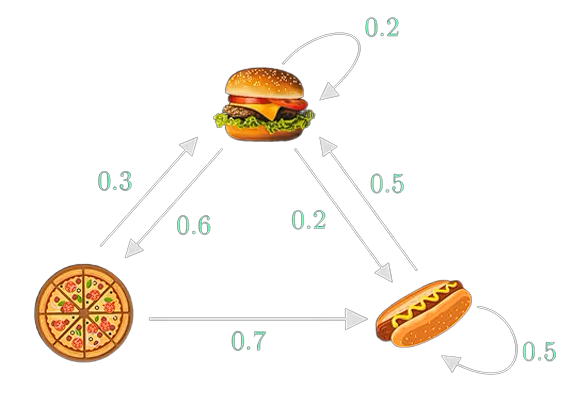
P(X_{n+1}=x|X_n = x_n)
Markov chains

?
P(X_{n+1}=x|X_n = x_n)
P(X_4 = \, \, \, \,\,\,\,\,| X_3 = \,\,\,\,\,\,\,) = 0.7
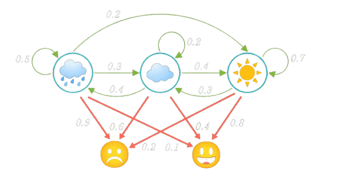
Hidden Markov Model
Hidden Markov Model

Hidden Markov Model
Hidden Markov Model
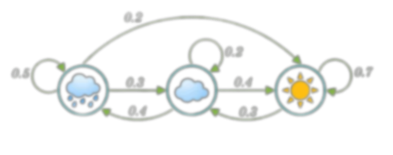
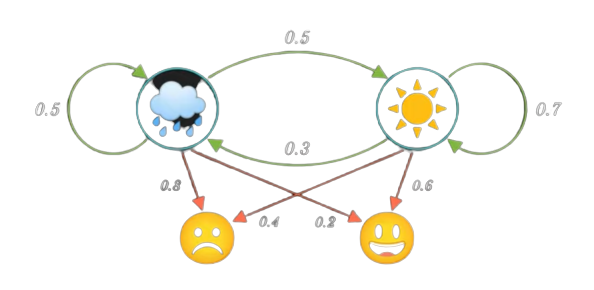
\text{States are hidden}
Hidden Markov Model
A = \,\,\,\,\,\,\,\,\,\begin{matrix}
0.5 & 0.3 & 0.2 \\
0.4 & 0.2 & 0.4 \\
0.0 & 0.3 & 0.7
\end{matrix}
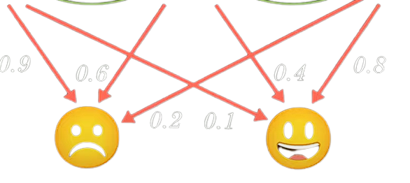
B = \,\,\,\,\,\,\,\,\,\begin{matrix}
0.9 & 0.1 \\
0.6 & 0.4 \\
0.2 & 0.8
\end{matrix}


Transition\,Matrix
Emission\,Matrix
Hidden Markov Model
Initial\,distribution
Stationary\,distribution
\pi = [0.3\,\,\,0.2\,\,\,0.5]
\pi = \pi A^n
\lim{n \rightarrow \infty}
\pi \rightarrow \pi^*
Hidden Markov Model
1.\,\,\text{Given a Hidden Markov Model and an observation sequence} \\
\text{What is the probability of the Model producing that particular sequence }
Problems
2.\,\,\text{Given a Hidden Markov Model and an observation sequence} \\
\text{Which state sequence maximize the probability of given observation sequence }
3.\,\,\text{Given an observation sequence ,how to train the model to get } \\
\text{such parameters of HMM to maximize the propability of observations sequence }
Problem 1
Problem 1
1.\,\,\text{Given a Hidden Markov Model and an observation sequence} \\
\text{What is the probability of the Model producing that particular sequence }
P(\,\,\,\,\,\,\,\,\,\,\,\,\,\,\,\,\,\,\,\,\,\,\,\,\,\,|\lambda) = ?
\lambda = {A\,\,\, \\
B\,\,\,\, \\
\pi
}
Forward Algorithm
Forward Algorithm
S
S
S
R
R
R
\pi = [0.375\,\,\,\,0.625]
Forward Algorithm
S
S
S
R
R
R
\pi = [0.375\,\,\,\,0.625]
\alpha_1(R) = 0.375\times0.8
\alpha_1(S) = 0.625\times0.4
Forward Algorithm
S
S
S
R
R
R
\pi = [0.375\,\,\,\,0.625]
\alpha_1(R)=0.3
\alpha_1(S) = 0.25
\alpha_2(R) = \alpha_1(R)\times0.5\times0.8 + \alpha_1(S)\times0.3\times0.8
\alpha_2(S) = \alpha_1(R)\times0.5\times0.4 + \alpha_1(S)\times0.7\times0.4
Forward Algorithm
S
S
S
R
R
R
\pi = [0.375\,\,\,\,0.625]
\alpha_1(R)=0.3
\alpha_2(S) = 0.25
\alpha_2(R) = 0.18
\alpha_2(S) = 0.13
\alpha_3(R) = 0.0258
\alpha_3(S) = 0.1086
Forward Algorithm
S
S
S
R
R
R
\alpha_1(R)=0.3
\alpha_2(S) = 0.25
\alpha_2(R) = 0.18
\alpha_2(S) = 0.13
\alpha_3(R) = 0.0258
\alpha_3(S) = 0.1086
P(\,\,\,\,\,\,\,\,\,\,\,\,\,\,\,\,\,\,\,\,\,\,\,\,\,\,|\lambda) = \alpha_3(R)+\alpha_3(S) = 0.1343
\lambda = {A\,\,\, \\
B\,\,\,\, \\
\pi
}
Problem 2
Problem 2
2.\,\,\text{Given a Hidden Markov Model and an observation sequence} \\
\text{Which state sequence maximize the probability of given observation sequence }
Problem 2
2.\,\,\text{Given a Hidden Markov Model and an observation sequence} \\
\text{Which state sequence maximize the probability of given observation sequence }
\begin{aligned}
& \underset{state\, seq}{\text{maximize}}
& & P(state \,seq|obs. \,seq, \lambda) \\
\end{aligned}
Problem 2
\begin{aligned}
& \underset{state\, seq}{\text{maximize}}
& & P(state \,seq|obs. \,seq, \lambda) \\
\end{aligned}
P(?|\,\,\,\,\,\,\,\,\,\,\,\,\,\,\,\,\,\,\,\,\,\,\, , \lambda)
Problem 2
P(?|\,\,\,\,\,\,\,\,\,\,\,\,\,\,\,\,\,\,\,\,\,\,\, , \lambda)
Solution
Viterbi Algorithm
Veterbi Algorithm
S
S
S
R
R
R
\pi = [0.375\,\,\,\,0.625]
Veterbi Algorithm
S
S
S
R
R
R
\pi = [0.375\,\,\,\,0.625]
\alpha_1(R) = 0.375\times0.8
\alpha_1(S) = 0.625\times0.4
Veterbi Algorithm
S
S
S
R
R
R
\alpha_1(R) = 0.3
\alpha_1(S) = 0.25
Veterbi Algorithm
S
S
S
R
R
R
\alpha_1(R) = 0.3
\alpha_1(S) = 0.25
Veterbi Algorithm
S
S
R
R
R
\alpha_1(R) = 0.3
Veterbi Algorithm
S
S
R
R
R
\alpha_1(R) = 0.3
0.12
0.06
Veterbi Algorithm
S
R
R
R
\alpha_1(R) = 0.3
0.12
Veterbi Algorithm
S
R
R
R
\alpha_1(R) = 0.3
0.012
0.036
0.12
Veterbi Algorithm
S
R
R
\alpha_1(R) = 0.3
0.036
0.12
Veterbi Algorithm
S
R
R
\alpha_1(R) = 0.3
0.12
0.036
Veterbi Algorithm
S
R
R
\alpha_1(R) = 0.3
0.12
0.036
P(?|\,\,\,\,\,\,\,\,\,\,\,\,\,\,\,\,\,\,\,\,\,\,\, , \lambda)
Veterbi Algorithm
P(R,R,S|\,\,\,\,\,\,\,\,\,\,\,\,\,\,\,\,\,\,\,\,\,\,\, , \lambda) = 0.036
Problem 3
O_1 , O_2 \cdots O_3
O_1 , O_2 \cdots O_i \cdots O_T
A^*,B^*,\pi^*
?
O_1
A^*,B^*,\pi^*
O_2
O_3
O_{T-2}
O_{T-1}
O_T
O_t
O_1
A^*,B^*,\pi^*
O_2
O_3
O_{T-2}
O_{T-1}
O_T
O_t
\alpha_t(i)=P\left( O_1 , O_2, \cdots O_t , q_t = S_i | \lambda \right)
S_i
O_1
A^*,B^*,\pi^*
O_2
O_3
O_{T-2}
O_{T-1}
O_T
O_t
\beta_t(i)=P\left( O_{t+1} , O_{t+2} , \cdots O_T , q_t = S_i | \lambda \right)
S_i
O_1
A^*,B^*,\pi^*
O_2
O_3
O_{T-2}
O_{T-1}
O_T
O_t
\gamma_t(i)=P\left( q_t = S_i |O, \lambda \right)
S_i
O_1
A^*,B^*,\pi^*
O_2
O_3
O_{T-2}
O_{T-1}
O_T
O_t
\xi_t(i,j)=P\left( q_t = S_i, q_{t+1} = S_j |O, \lambda \right)
S_i
S_j
O_{t+1}
O_1
A^*,B^*,\pi^*
O_2
O_3
O_{T-2}
O_{T-1}
O_T
O_t
\xi_t(i,j)=P\left( q_t = S_i, q_{t+1} = S_j |O, \lambda \right)
S_i
S_j
O_{t+1}
\alpha_t(i)
\beta_{t+1}(j)
a_{ij}b_j(O_{t+1})
O_1
A^*,B^*,\pi^*
O_2
O_3
O_{T-2}
O_{T-1}
O_T
O_t
\xi_t(i,j)=
S_i
S_j
O_{t+1}
\alpha_t(i)
\beta_{t+1}(j)
a_{ij}b_j(O_{t+1})
O_1
A^*,B^*,\pi^*
O_2
O_3
O_{T-2}
O_{T-1}
O_T
O_t
\xi_t(i,j)=
S_i
S_j
O_{t+1}
\alpha_t(i)
\beta_{t+1}(j)
a_{ij}b_j(O_{t+1})
\frac{\alpha_t(i)a_{ij}b_j(O_{t+1})\beta_{t+1}(j)}{P(O| \lambda)}
O_1
A^*,B^*,\pi^*
O_2
O_3
O_{T-2}
O_{T-1}
O_T
O_t
\xi_t(i,j)=
S_i
S_j
O_{t+1}
\alpha_t(i)
\beta_{t+1}(j)
a_{ij}b_j(O_{t+1})
\frac{\alpha_t(i)a_{ij}b_j(O_{t+1})\beta_{t+1}(j)}{P(O| \lambda)}
\sum_{t}
S_i
S_j
S_i
S_j
O_1
A^*,B^*,\pi^*
O_2
O_3
O_{T-2}
O_{T-1}
O_T
O_t
\xi_t(i,j)=
S_i
S_j
O_{t+1}
\frac{\alpha_t(i)a_{ij}b_j(O_{t+1})\beta_{t+1}(j)}{P(O| \lambda)}
\sum_{t}^{T}
S_i
S_j
S_i
S_j
E[a_{ij}]
E[a_{ij}]
Expected Number of Transitions
From State i to j
i,j
i,j
O_1
A^*,B^*,\pi^*
O_2
O_3
O_{T-2}
O_{T-1}
O_T
O_t
\gamma_t(i)= \sum_t P\left( q_t = S_i |O, \lambda \right)
S_i
E[a_{ij}]
j
E[a_{ij}]
j
Expected Number of transitions from state Si
A^*
B^*
\pi^*
a_{ij} = \frac{E\left [ S_i \rightarrow S_j \right] }{E[S_i \rightarrow]}
a_{ij} = \frac{\sum_{t} \xi_t(i,j)}{\sum_t \gamma_t(i)}
A^*
B^*
\pi^*
b_i(k) = \frac{E [S_i \cap O_k] }{E[S_i]}
\frac{}{\sum_t \gamma_t(i)}
\sum_t \gamma_t(i)
O_t = O_k
b_i(k)=
\gamma_t(i)= \sum_t P\left( q_t = S_i |O, \lambda \right)
Iteratively Calculate A,B
a_{ij} = \frac{\sum_{t} \xi_t(i,j)}{\sum_t \gamma_t(i)}
\frac{}{\sum_t \gamma_t(i)}
\sum_t \gamma_t(i)
O_t = O_k
b_i(k)=
A
B
Converges to a local maxima
Iteratively Calculate A,B
a_{ij} = \frac{\sum_{t} \xi_t(i,j)}{\sum_t \gamma_t(i)}
\frac{}{\sum_t \gamma_t(i)}
\sum_t \gamma_t(i)
O_t = O_k
b_i(k)=
A
B
Converges to a local maxima
Baum Welch Algorithm, is a type of Expectation Maximisation
Credit Card fraud detection
Credit Card fraud detection

Credit Card fraud detection
₹100
₹200
₹500
₹1000
₹7000
L
L
M
M
H
Credit Card fraud detection
₹100
₹200
₹500
₹1000
₹7000
L
L
M
M
H
L
L
M
M
H
Observation
Seq.
Credit Card fraud detection
₹100
₹200
₹500
₹1000
₹7000
L
L
M
M
H
L
L
M
M
H
P(L | O) = \frac{2}{5}
P(M | O) = \frac{2}{5}
P(H | O) = \frac{1}{5}
Credit Card fraud detection
₹100
₹200
₹500
₹1000
₹7000
L
L
M
M
H
L
L
M
M
H
P(L | O) = \frac{2}{5}
P(M | O) = \frac{2}{5}
P(H | O) = \frac{1}{5}
Naively We can Observe, Given the observation sequence,Probability of a high transaction is low
Credit Card fraud detection
₹100
₹200
₹500
₹1000
₹7000
L
L
M
M
H
L
L
M
M
H
What if, we can learn from history?
The Process can be modeled as a Markov Process
The Process can be modeled as a Markov Process
Further, Since we aren't sure about the states causing the Observation,It should be modelled as Hidden Markov Model
Learning...Hmm....?🤔
O_1 , O_2 \cdots O_i \cdots O_T
A^*,B^*,\pi^*
?
Baum Welch Algorithm comes to the rescue
O_1 , O_2 \cdots O_i \cdots O_T
A^*,B^*,\pi^*
?
After Learning the Parameters of HMM, We can find the probability of a sequence of observations, Given the Model which is our Forward Algorithm
A^*,B^*,\pi^*
O_1 , O_2 \cdots O_i \cdots O_T
A^*,B^*,\pi^*
Credit Card fraud detection
₹100
₹200
₹500
₹1000
₹7000
₹20000
19MAT117
Applications and Future Learning Directions
Applications
- Sequence Alignment in Biology
- Widely Used in NLP
- Inference from Time Series
- Molecular Evolutionary models
- Phylogenitcs
Applications
Future Learning Directions
- Generalizations of HMM - Bayesian Networks
- Continuous-Time Markov Models
- Other methods of Expectation-Maximization for learning
References
[3] djp3, Hidden Markov Models 12: the Baum-Welch algorithm, (Apr. 10, 2020). Accessed: Jan. 17, 2022. [Online]. Available: https://www.youtube.com/watch?v=JRsdt05pMoI
[5] “Markov Chains Clearly Explained! - YouTube.” https://www.youtube.com/ (accessed Jan. 17, 2022).
[4] Normalized Nerd, Hidden Markov Model Clearly Explained! Part - 5, (Dec. 26, 2020). Accessed: Jan. 17, 2022. [Online]. Available: https://www.youtube.com/watch?v=RWkHJnFj5rY
[2] L. R. Rabiner, “A tutorial on hidden Markov models and selected applications in speech recognition,” Proceedings of the IEEE, vol. 77, no. 2, pp. 257–286, Feb. 1989, doi: 10.1109/5.18626.
[1] “(14) (PDF) A revealing introduction to hidden markov models.” https://www.researchgate.net/publication/288957333_A_revealing_introduction_to_hidden_markov_models (accessed Jan. 17, 2022).
Thank you Mam
MIS-3
By Incredeble us


