Deep Learning for Signal and Image Processing
Team 01
Assignment 1a,1b,1c
Assignment 1a
Dataset Familiarization
Assignment 1a
Dataset Familiarization
Python program to load the iris data from a given CSV file into a data frame (data_iris)
import pandas as pd
import matplotlib.pyplot as plt

# Load the iris data from a given CSV file into a data frame (data_iris)
data_iris = pd.read_csv('/content/iris.csv')
Assignment 1a
Dataset Familiarization
Python program to load the iris data from a given CSV file into a data frame (data_iris)
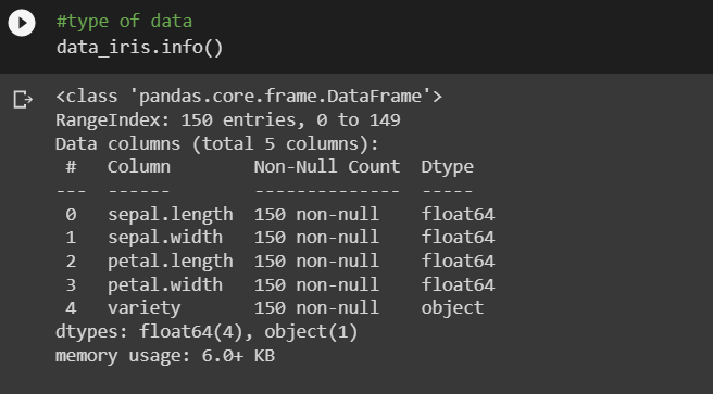
Shape of data
Type of data

Assignment 1a
Dataset Familiarization
Python program to load the iris data from a given CSV file into a data frame (data_iris)
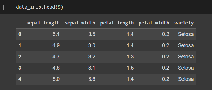
first 5 rows with labels
Find the keys
Not Applicable, since we loadded the data from csv file. However, sklearns load data gives the result in a dict
Assignment 1a
Dataset Familiarization
Python program to load the iris data from a given CSV file into a data frame (data_iris)
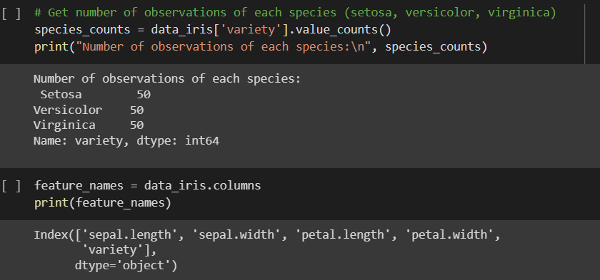
find number of features and feature names
Assignment 1a
Dataset Familiarization
Python program to load the iris data from a given CSV file into a data frame (data_iris)
Description of Iris data
The iris dataset is a classic multivariate dataset used for classification and data analysis. It contains measurements of various attributes of three different species of iris flowers: Setosa, Versicolor, and Virginica. The measurements include the length and width of the sepals and petals, in centimeters.
The dataset consists of 150 samples, with 50 samples per species, and is widely used in machine learning and statistical analysis as a benchmark dataset. It was first introduced in 1936 by the British statistician and biologist Ronald Fisher, and has since become a popular example in the fields of pattern recognition, data visualization, and exploratory data analysis.
Assignment 1a
Dataset Familiarization
Python program to load the iris data from a given CSV file into a data frame (data_iris)
number of categories/class labels in the data
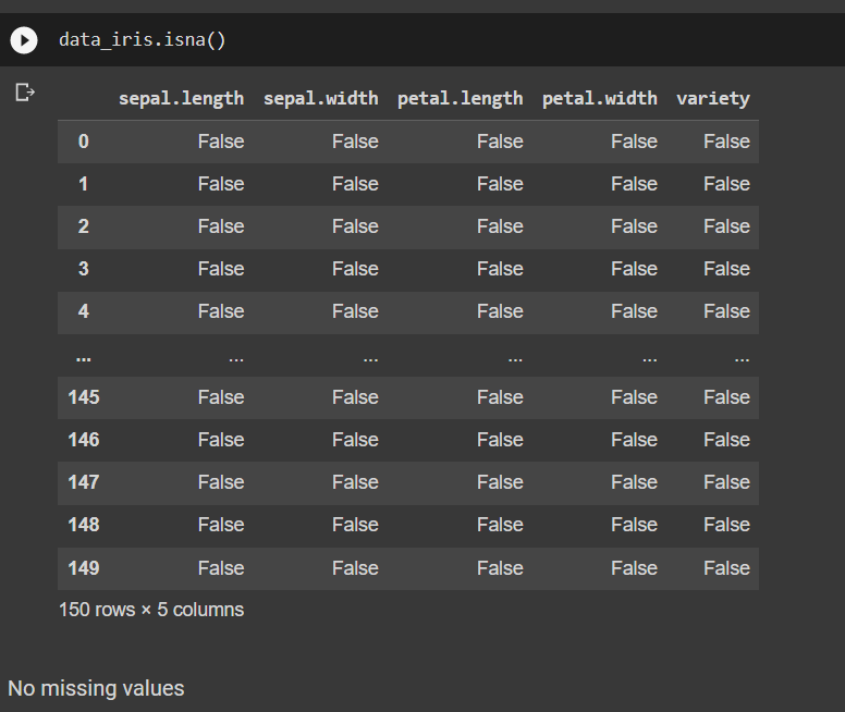
get the missing values and nan values (with feature and class label indexing).
Assignment 1a
Dataset Familiarization
Python program to load the iris data from a given CSV file into a data frame (data_iris)
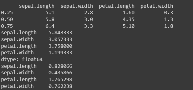
view basic statistical details like percentile, mean, std etc. of iris data
percentiles = data_iris.quantile([0.25, 0.5, 0.75])

mean = data_iris.mean()

std_dev = data_iris.std()

print(percentiles)
print(mean)
print(std_dev)
Assignment 1a
Dataset Familiarization
Python program to load the iris data from a given CSV file into a data frame (data_iris)
view basic statistical details like percentile, mean, std etc. of iris data
Assignment 1a
Dataset Familiarization
Python program to load the iris data from a given CSV file into a data frame (data_iris)
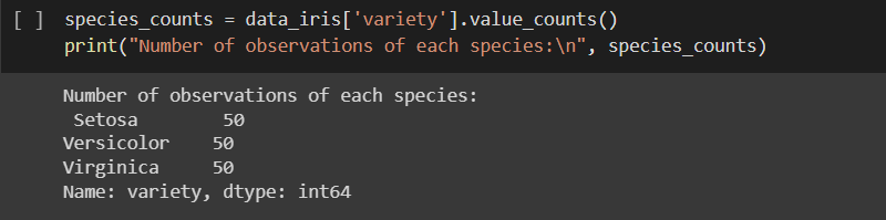
get number of observations of each species (setosa, versicolor, virginica) from iris data and create sub data frames for each species (data_iris_setosa, data_iris_versicolor, data_iris_virginica)
# Create sub data frames for each species
data_iris_setosa = data_iris[data_iris['variety'] == 'Setosa']
data_iris_versicolor = data_iris[data_iris['variety'] == 'Versicolor']
data_iris_virginica = data_iris[data_iris['variety'] == 'Virginica']
Assignment 1a
Dataset Familiarization
Python program to load the iris data from a given CSV file into a data frame (data_iris)
drop Id column from data_iris Dataframe and create a new data frame with this modified part.
data_iris_modified = data_iris.drop(columns=['variety']).reset_index()create two date frames data_iris_feature (only with feature columns) and data_iris_species (only with species column). create a Bar plot and a Pie plot to get the frequency of the three species of the Iris data create a graph to find the relationship between the sepal length and sepal width of different species (scatter plot , give different color labels for different species)
# Create two date frames data_iris_feature (only with feature columns) and data_iris_species (only with species column)
data_iris_species = data_iris['variety']
# Create a Bar plot to get the frequency of the three species of the Iris data
species_counts.plot(kind='bar')
plt.title('Frequency of Iris species')
plt.xlabel('Species')
plt.ylabel('Frequency')
plt.show()
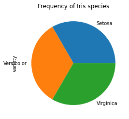
# Create a Pie plot to get the frequency of the three species of the Iris data
species_counts.plot(kind='pie')
plt.title('Frequency of Iris species')
plt.show()
Assignment 1a
Dataset Familiarization
Python program to load the iris data from a given CSV file into a data frame (data_iris)
create a Bar plot and a Pie plot to get the frequency of the three species of the Iris data.
# Create two date frames data_iris_feature (only with feature columns) and data_iris_species (only with species column)
data_iris_species = data_iris['variety']


# Create a Bar plot to get the frequency of the three species of the Iris data
species_counts.plot(kind='bar')
plt.title('Frequency of Iris species')
plt.xlabel('Species')
plt.ylabel('Frequency')
plt.show()

# Create a Pie plot to get the frequency of the three species of the Iris data
species_counts.plot(kind='pie')
plt.title('Frequency of Iris species')
plt.show()
Assignment 1a
Dataset Familiarization
Python program to load the iris data from a given CSV file into a data frame (data_iris)
create a Bar plot and a Pie plot to get the frequency of the three species of the Iris data.
# Create two date frames data_iris_feature (only with feature columns) and data_iris_species (only with species column)
data_iris_species = data_iris['variety']


# Create a Bar plot to get the frequency of the three species of the Iris data
species_counts.plot(kind='bar')
plt.title('Frequency of Iris species')
plt.xlabel('Species')
plt.ylabel('Frequency')
plt.show()

# Create a Pie plot to get the frequency of the three species of the Iris data
species_counts.plot(kind='pie')
plt.title('Frequency of Iris species')
plt.show()

Assignment 1a
Dataset Familiarization
Python program to load the iris data from a given CSV file into a data frame (data_iris)
create a graph to find the relationship between the sepal length and sepal width of different species (scatter plot , give different color labels for different species)
# Create two date frames data_iris_feature (only with feature columns) and data_iris_species (only with species column)
data_iris_species = data_iris['variety']


# Create a Bar plot to get the frequency of the three species of the Iris data
species_counts.plot(kind='bar')
plt.title('Frequency of Iris species')
plt.xlabel('Species')
plt.ylabel('Frequency')
plt.show()

# Create a Pie plot to get the frequency of the three species of the Iris data
species_counts.plot(kind='pie')
plt.title('Frequency of Iris species')
plt.show()
# Create a graph to find the relationship between the sepal length and sepal width of different species (scatter plot, give different color labels for different species)
plt.scatter(data_iris_setosa['sepal.length'], data_iris_setosa['sepal.width'], color='red', label='Iris-setosa')
plt.scatter(data_iris_versicolor['sepal.length'], data_iris_versicolor['sepal.width'], color='green', label='Iris-versicolor')
plt.scatter(data_iris_virginica['sepal.length'], data_iris_virginica['sepal.width'], color='blue', label='Iris-virginica')
plt.title('Relationship between sepal length and sepal width of Iris species')
plt.xlabel('Sepal length')
plt.ylabel('Sepal width')
plt.legend()
plt.show()
Assignment 1a
Dataset Familiarization
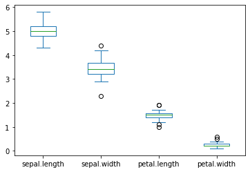
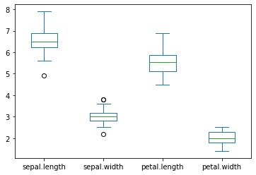
create a graph to see how the feature (SepalLength, SepalWidth, PetalLength, PetalWidth) are distributed for each species. Comment on it.
# Create two date frames data_iris_feature (only with feature columns) and data_iris_species (only with species column)
data_iris_species = data_iris['variety']


# Create a Bar plot to get the frequency of the three species of the Iris data
species_counts.plot(kind='bar')
plt.title('Frequency of Iris species')
plt.xlabel('Species')
plt.ylabel('Frequency')
plt.show()

# Create a Pie plot to get the frequency of the three species of the Iris data
species_counts.plot(kind='pie')
plt.title('Frequency of Iris species')
plt.show()
Setosa
versicolor
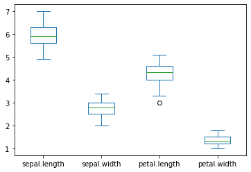
virginica
Assignment 1a
Dataset Familiarization
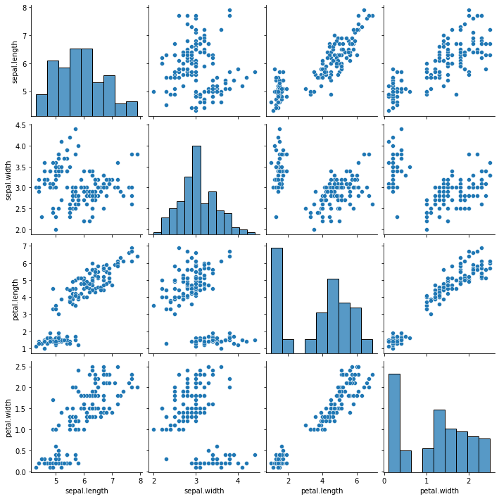
create a pairplot of the iris data set and check which flower speciesseems to be the most separable. Comment on it.
# Create two date frames data_iris_feature (only with feature columns) and data_iris_species (only with species column)
data_iris_species = data_iris['variety']


# Create a Bar plot to get the frequency of the three species of the Iris data
species_counts.plot(kind='bar')
plt.title('Frequency of Iris species')
plt.xlabel('Species')
plt.ylabel('Frequency')
plt.show()

# Create a Pie plot to get the frequency of the three species of the Iris data
species_counts.plot(kind='pie')
plt.title('Frequency of Iris species')
plt.show()
Assignment 1a
Dataset Familiarization
find the correlation between variables of iris data (between features and between feature and species). Also create a heatmap using Seaborn to present their relations
# Create two date frames data_iris_feature (only with feature columns) and data_iris_species (only with species column)
data_iris_species = data_iris['variety']


# Create a Bar plot to get the frequency of the three species of the Iris data
species_counts.plot(kind='bar')
plt.title('Frequency of Iris species')
plt.xlabel('Species')
plt.ylabel('Frequency')
plt.show()

# Create a Pie plot to get the frequency of the three species of the Iris data
species_counts.plot(kind='pie')
plt.title('Frequency of Iris species')
plt.show()

data_iris_modified= data_iris_modified.drop(["index"],axis=1)
correlation = data_iris_modified.corr()
sns.heatmap(correlation)
Assignment 1b
Linear Regression
Assignment 1b
Linear Regression
Create a complete document on Linear Regression model representation cost function Gradient descent algorithm Python program for linear regression (single and multi-variable)
Assignment 1b
Linear Regression(Simple)
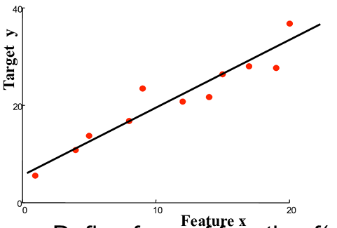
Evaluate line y = mx+c
where, m is the slope of the line
c is the y_intercept
Assignment 1b
Linear Regression(Simple)
Evaluate line y = mx+c
where, m is the slope of the line
c is the y_intercept
Assignment 1b
Linear Regression(Multivariate)
\hat{y}(x)=\theta_{0}+\theta_{1} x_{1}+\theta_{2} x_{2}+\ldots+\theta_{n} x_{n}
This can be represented in Matrix-Vector Form as
\hat{y}(x)=\theta x_{n}^{T} \\
\theta=\left[\theta_{0}, \ldots, \theta_{n}\right] \\ x=\left[1, x_{1}, \ldots, x_{n}\right]
Our aim now is to learn Theta Vector
Assignment 1b
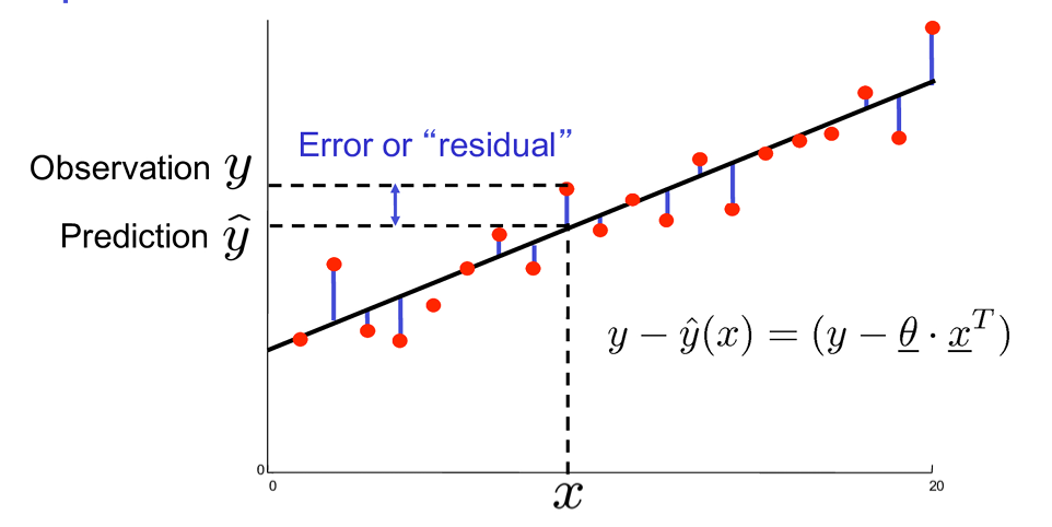
Geometrical Meaning: Optimization POV
Assignment 1b
Geometrical Meaning: Optimization POV
Cost Function
J(\theta) = \frac{1}{2m} \sum_{i=1}^m (h_\theta(x^{(i)}) - y^{(i)})^2
where m is the number of training examples, h() is the predicted value for the i-th example, and y^i is the actual value for the i-th example.
Assignment 1b
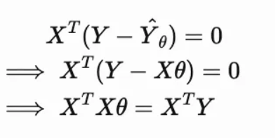
Geometrical Meaning: Linear Algebra POV

Assignment 1b
# Importing the libraries
import pandas as pd
import numpy as np
import matplotlib.pyplot as plt
from sklearn.linear_model import LinearRegression,SGDRegressor
from sklearn.metrics import mean_squared_error, r2_score

# Load dataset
data = pd.read_csv("data.csv")

train_data = data.sample(frac=0.75, random_state=1)
test_data = data.drop(train_data.index)

# linear regression model
regressor = LinearRegression()
#To explicitly use SGD
regressor = SGDRegressor()

# fitting
regressor.fit(train_data[['x']], train_data['y'])

# predicting
y_pred = regressor.predict(test_data[['x']])

# Evaluate
mse = mean_squared_error(test_data['y'], y_pred)
rmse = np.sqrt(mse)
r2 = r2_score(test_data['y'], y_pred)

print("MSE: ", mse)
print("RMSE: ", rmse)
print("R2: ", r2)
Assignment 1b

Assignment 1b
Draw a performance plot of the regression model(% of training data vs RMSE)
import numpy as np
import pandas as pd
import matplotlib.pyplot as plt

# function to calculate RMSE
def rmse(y_true, y_pred):
    return np.sqrt(np.mean((y_true - y_pred) ** 2))

  train_sizes = np.arange(0.1, 1.0, 0.1)

# To store rmse values
rmse_values = []

# Parse through the training data
for train_size in train_sizes:

    # perform linear regression on training size
    n = len(data)
    train_size = int(n * train_size)
    X_train, y_train = X[:train_size], y[:train_size]
    X_test, y_test = X[train_size:], y[train_size:]

    X_train_norm = (X_train - np.mean(X_train)) / np.std(X_train)
    y_train_norm = (y_train - np.mean(y_train)) / np.std(y_train)
    X_train_norm = np.c_[np.ones((len(X_train_norm), 1)), X_train_norm]
    optimised = np.linalg.inv(X_train_norm.T.dot(X_train_norm)).dot(X_train_norm.T).dot(y_train_norm)

    X_test_norm = (X_test - np.mean(X_train)) / np.std(X_train)
    X_test_norm = np.c_[np.ones((len(X_test_norm), 1)), X_test_norm]
    y_pred_norm = X_test_norm.dot(optimised)

    y_pred = y_pred_norm * np.std(y_train) + np.mean(y_train)

    rmse_values.append(rmse(y_test, y_pred))

# Plot
plt.plot(train_sizes, rmse_values)
plt.xlabel('% of training data')
plt.ylabel('RMSE')
plt.title('Performance of linear regression model')
plt.show()
Assignment 1b
Draw a performance plot of the regression model(% of training data vs RMSE)

Assignment 1c
Logistic Regression
Assignment 1c
Logistic Regression
Assignment 1c
Logistic Regression
\Sigma
\int
\hat{y}
x_1
w_1
x_3
x_2
w_2
w_3
Assignment 1c
Logistic Regression
\Sigma
\int
\hat{y}
x_1
w_1
x_3
x_2
w_2
w_3
Assignment 1c
Logistic Regression
1
0.5
3
2
0.2
0.4
\hat{y}
g(z)
x = \begin{bmatrix} 1 \\ 2 \\ 3 \end{bmatrix} \\
y = 1 \\
\text{random weights , } \\
w = \begin{bmatrix} 0.5 \\ 0.2 \\ 0.4 \end{bmatrix} \\
z = w^T \cdot x
[1 \cdot 0.5 + 2 \cdot 0.2 + 3 \cdot 0.4]
\text{z = 2.1}
Assignment 1c
Logistic Regression
\text{Activation Function}
Sigmoid Function

g(z) = \frac{1}{1 + e^{-z} }
g'(z) = g(z) \cdot (1 - g(z) )
Assignment 1c
Logistic Regression
g(z) = \frac{1}{1 + e^{-z} }
1
0.5
3
2
0.2
0.4
g(z)
\text{z = 2.1}
\hat{y} = 0.8909
Assignment 1c
Logistic Regression
g(z) = \frac{1}{1 + e^{-z} }
1
0.5
3
2
0.2
0.4
g(z)
\text{z = 2.1}
\hat{y} = 0.8909
OOPs! 🤥
Wasn't the true output 1?
We Should Punish the Network , so
It Behaves Properly
LOSS FUNCTIONS
Answer:
Assignment 1c
Logistic Regression
LOSS FUNCTIONS
Binary Cross Entropy Loss
L(y , \hat{y}) = - y \cdot log(\hat{y} ) - (1-y) \cdot log(1 - \hat{y})
L(y , \hat{y} ) = \begin{cases}
- log(\hat{y}) && y == 1 \\
- log(1 - \hat{y}) && y == 0
\end{cases}
Assignment 1c
Logistic Regression
w = w + (-1) \cdot \alpha (\frac{\partial L(y,\hat{y} )}{\partial w})
\alpha \rightarrow scalar \rightarrow Learning \, Rate
Assignment 1c
Logistic Regression

Assignment 1c
Logistic Regression
1
0.5
3
2
0.2
0.4
g(z)
\text{z = 2.1}
\hat{y} = 0.8909
L(1 , 0.8009) = - 1 \cdot log(0.8909) - (1-1) \cdot log(1 - 0.8909)
Assignment 1c
Logistic Regression
1
0.5
3
2
0.2
0.4
g(z)
\text{z = 2.1}
\hat{y} = 0.8909
L(1 , 0.8009) = 0.1155
Assignment 1c
Logistic Regression
1
0.5
3
2
0.2
0.4
\text{z = 2.1}
\hat{y} = 0.8909
L(1 , 0.8009) = 0.1155
\frac{\partial L}{\partial \hat{y} }
\frac{\partial L}{\partial \hat{y}} = \frac{-y}{\hat{y}} + \frac{1 - y}{1 - \hat{y}}
\frac{ \partial L(1 , 0.8909) }{ \partial \hat{y}}= - \frac{1}{0.89} = -1.123
z
g(z)
Assignment 1c
Logistic Regression
1
0.5
3
2
0.2
0.4
\text{z = 2.1}
\hat{y} = 0.8909
L(1 , 0.8009) = 0.1155
\frac{\partial L}{\partial \hat{y} }=-1.123
z
g(z)
\frac{\partial L}{\partial z }
\frac{ \partial L} {\partial z} = \frac{\partial L}{\partial \hat{y}} \cdot \frac{\partial \hat{y}}{\partial z}
\left( -\frac{1} {\hat{y}} \right) \cdot \left( \hat{y} (1 - \hat{y}) \right)
-1.123 \cdot (0.8909(1-0.8909)) \\
= -0.1092
Assignment 1c
Logistic Regression
1
3
2
\text{z = 2.1}
\hat{y} = 0.8909
L(1 , 0.8009) = 0.1155
\frac{\partial L}{\partial \hat{y} }=-1.123
z
g(z)
\frac{\partial L}{\partial z } = -0.1092
\frac{\partial L}{\partial w_i} = \frac{\partial L}{\partial z} \cdot \frac{\partial z}{\partial w_i}
\frac{\partial z}{\partial w_i} =\frac{\partial \sum w_i x_i}{\partial w_i} = x_i
\frac{\partial L}{\partial w_1} = -0.1092*1 \\
\frac{\partial L}{\partial w_2} = -0.1092*2 \\
\frac{\partial L}{\partial w_3} = -0.1092*3 \\
\frac{\partial L}{\partial w_1}
\frac{\partial L}{\partial w_3}
\frac{\partial L}{\partial w_2}
Assignment 1c
Logistic Regression
\text{z = 2.1}
\hat{y} = 0.8909
L(1 , 0.8009) = 0.1155
\frac{\partial L}{\partial \hat{y} }=-1.123
\frac{\partial L}{\partial z } = -0.1092
\frac{\partial L}{\partial w_1} = -0.1092 \\
\frac{\partial L}{\partial w_2} = -0.2184 \\
\frac{\partial L}{\partial w_3} = -0.3276 \\
w_1 = w_1 - \alpha \cdot \frac{\partial L}{\partial w_1}
w_2 = w_2 - \alpha \cdot \frac{\partial L}{\partial w_2}
w_3 = w_3 - \alpha \cdot \frac{\partial L}{\partial w_3}
\alpha \rightarrow Learning \ rate
Assignment 1c
Logistic Regression
\text{z = 2.1}
\hat{y} = 0.8909
L(1 , 0.8009) = 0.1155
\frac{\partial L}{\partial \hat{y} }=-1.123
\frac{\partial L}{\partial z } = -0.1092
\frac{\partial L}{\partial w_1} = -0.1092 \\
\frac{\partial L}{\partial w_2} = -0.2184 \\
\frac{\partial L}{\partial w_3} = -0.3276 \\
\alpha \rightarrow Learning \ rate
w_1 = 0.5 - 1 \cdot (-0.1092)
w_2 = 0.2- 1 \cdot (-0.2184)
w_3 = 0.4- 1 \cdot (-0.3276)
Assignment 1c
Logistic Regression
x = \begin{bmatrix} 1 \\ 2 \\ 3 \end{bmatrix} \\
y = 1 \\
\text{updated weights , } \\
w = \begin{bmatrix} 0.6092 \\ 0.4184 \\ 0.7276 \end{bmatrix} \\
1
0.6092
3
2
0.4184
0.7276
\hat{y}
g(z)
z = w^T \cdot x
[1 \cdot 0.6092 + 2 \cdot 0.4184 + 3 \cdot 0.7276] \\
= 3.6288
g(z) = g(3.6288) = 0.9739
L(1, 0.9739) = 0.02
Old \ loss = 0.1155
Assignment 1c
Single, Binary Logistic Regression Using Inbuilt command
data = load_breast_cancer()
X = data.data[:, 0].reshape(-1, 1)  # Using only the first feature
y = data.target
X_train, X_test, y_train, y_test = train_test_split(X, y, test_size=0.25, random_state=42)
logreg = LogisticRegression()
logreg.fit(X_train, y_train)
y_pred = logreg.predict(X_test)
print(classification_report(y_test, y_pred))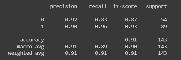
Assignment 1c
Single, Binary Logistic Regression
class Logistic_Regression:
    def __init__(self, lr=0.01, num_iter=100000, fit_intercept=True, verbose=False):
        self.lr = lr
        self.num_iter = num_iter
        self.fit_intercept = fit_intercept
        self.verbose = verbose

    def __add_intercept(self, X):
        intercept = np.ones((X.shape[0], 1))
        return np.concatenate((intercept, X), axis=1)

    def __compute_cost(self, h, y):
        epsilon = 1e-5
        m = y.shape[0]
        cost = (-1/m) * np.sum(y*np.log(h+epsilon) + (1-y)*np.log(1-h+epsilon))
        return cost

    def fit(self, X, y):
        if self.fit_intercept:
            X = self.__add_intercept(X)

        self.theta = np.zeros(X.shape[1])

        for i in range(self.num_iter):
            z = np.dot(X, self.theta)
            h = sigmoid(z)
            gradient = np.dot(X.T, (h-y)) / y.size
            self.theta -= self.lr * gradient

            if self.verbose and i % 10000 == 0:
                z = np.dot(X, self.theta)
                h = sigmoid(z)
                print(f'loss: {self.__compute_cost(h, y)} \t')

    def predict_prob(self, X):
        if self.fit_intercept:
            X = self.__add_intercept(X)

        return sigmoid(np.dot(X, self.theta))

    def predict(self, X, threshold=0.5):
        return self.predict_prob(X) >= threshold
Assignment 1c
Single, Binary Logistic Regression
model = Logistic_Regression(lr=0.1, num_iter=300000)
model.fit(X_train, y_train.values.ravel())

preds = model.predict(X_test)
print(classification_report(y_test, preds))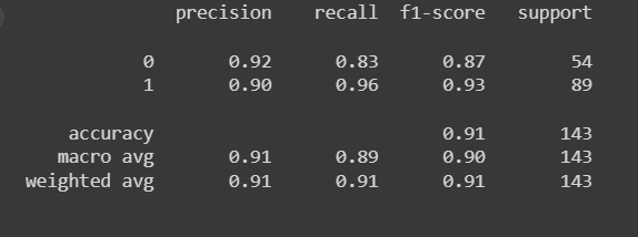
Assignment 1d
Random Forest and Decision Trees
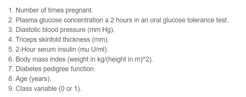
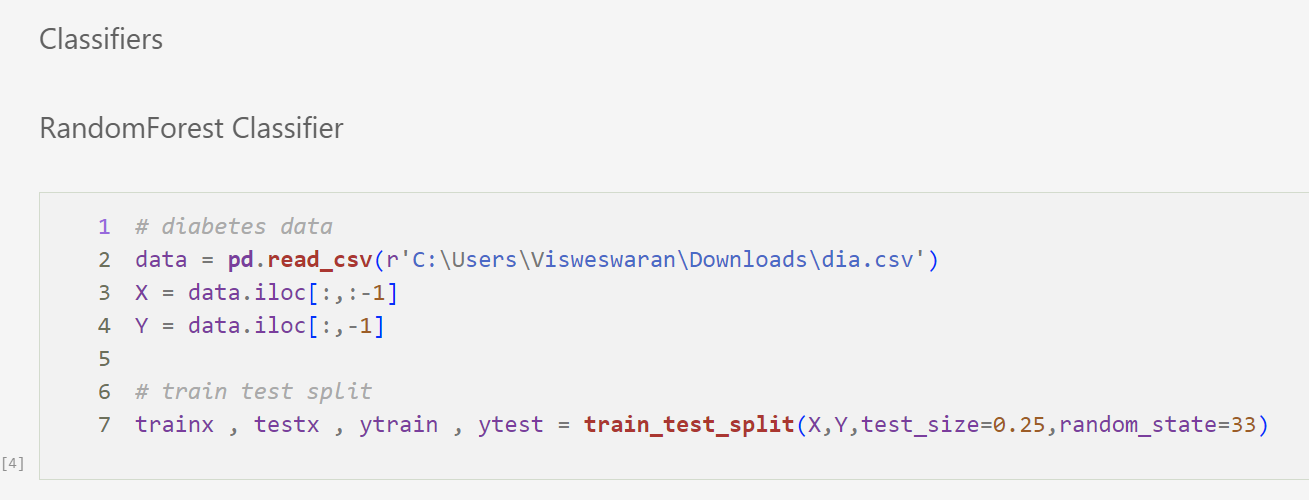
Classification Data
Given these information , predict if the person may get diabetes in the future
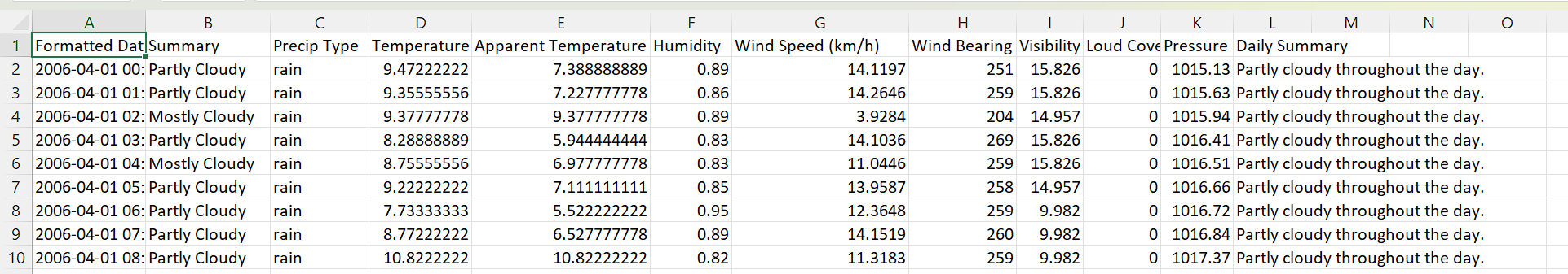
Regression Data
Given the information , predict the humidity for a given day
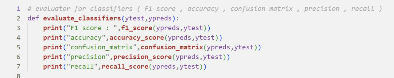
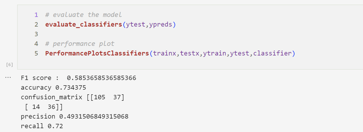
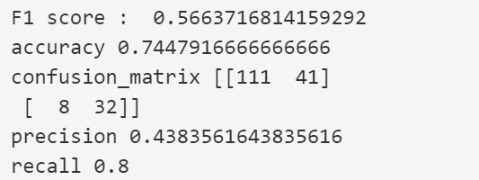
Evaluating Classifiers
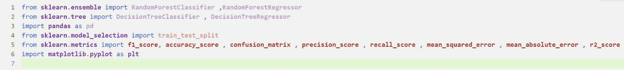
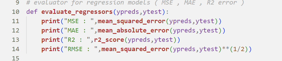
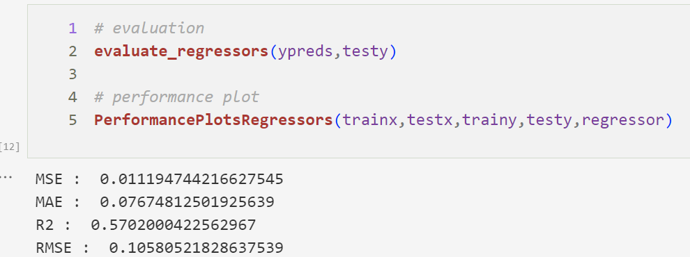
Evaluating Regressors
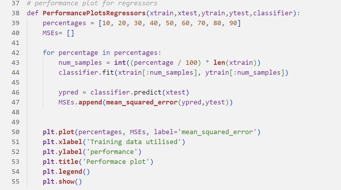
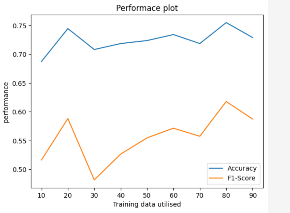
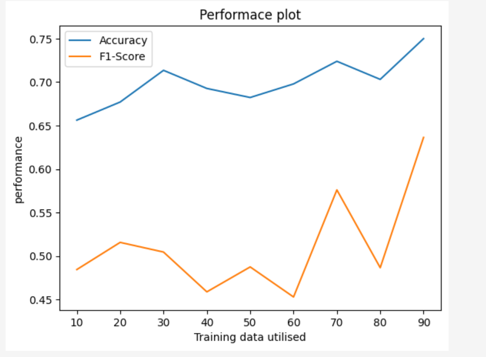
Performance plots
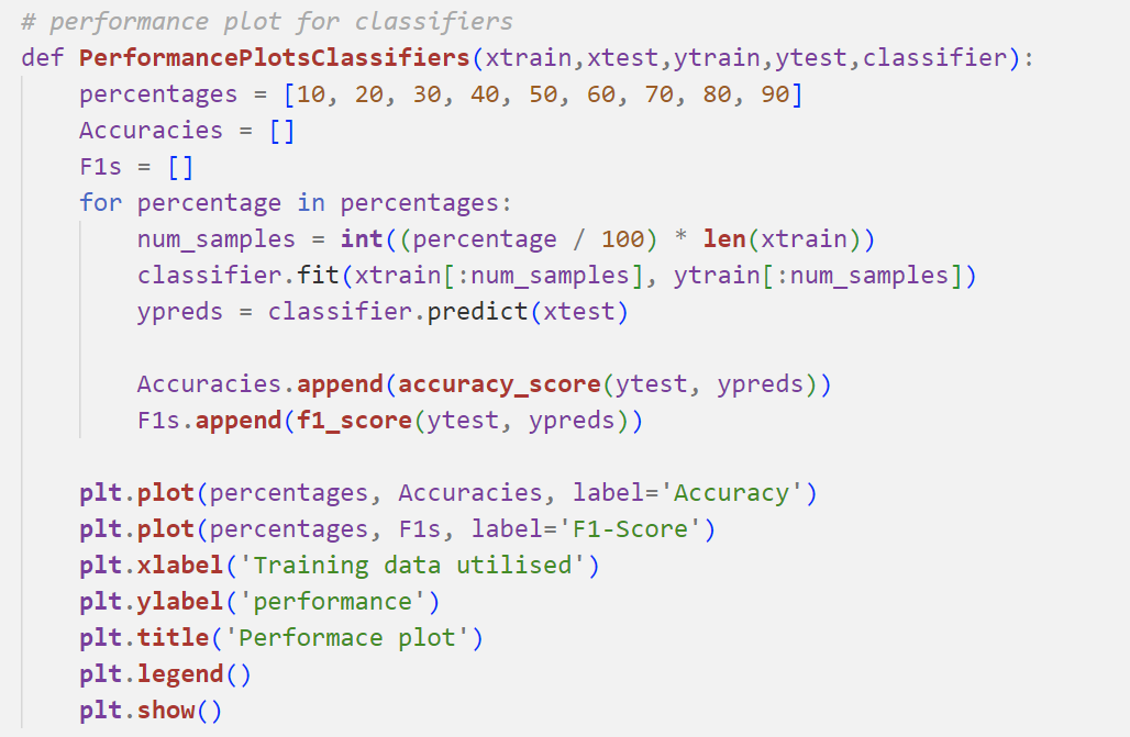
Performance plots
Random Forest Classifier
Random Forest Classifier
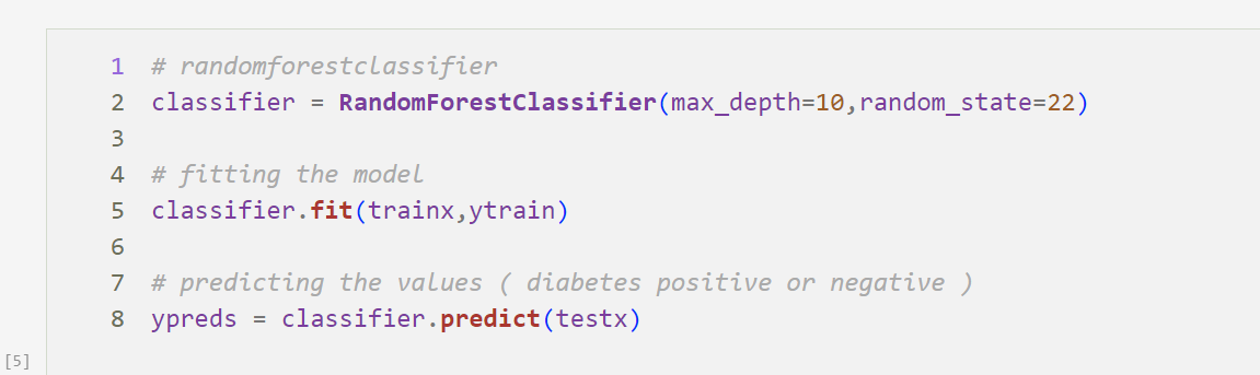
Random Forest Classifier
Random Forest Classifier Performance Plot
Decision Tree Classifier
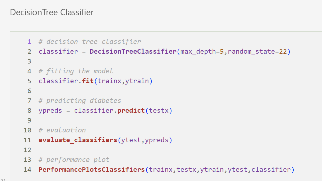
Decision Tree Classifier
Decision Tree Classifier Performance PLot
Random Forest Regression
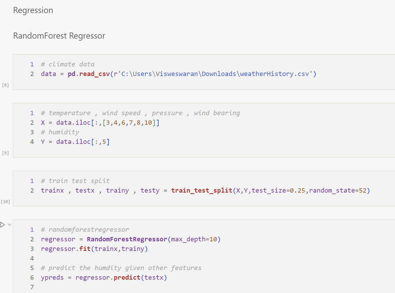
Random Forest Regression
Random Forest Regression Performance Plot
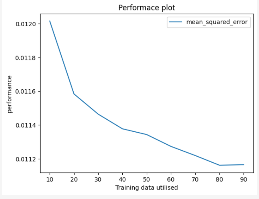
Decision Tree Regression
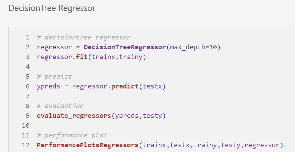
Decision Tree Regression
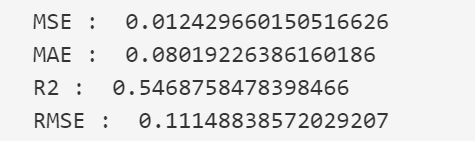
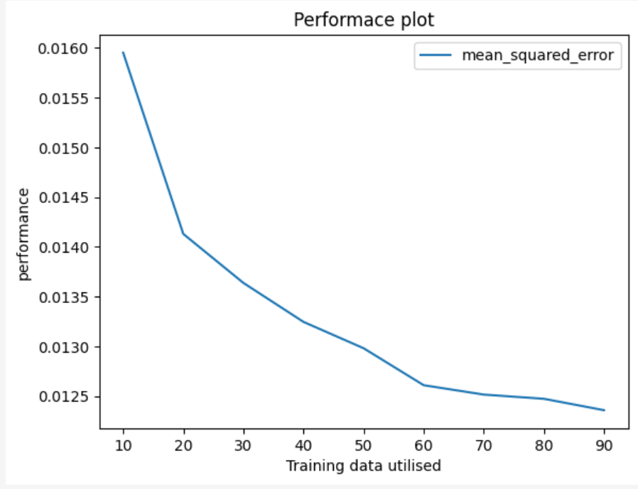
Decision Tree Regression Performance Plot
deck
By Incredeble us


