From Linear Systems to NNs
Aadharsh Aadhithya A
3x+4y=12
What does it mean?
3x+4y=12
What does it mean?
Set of all points (x,y) that satisfy the relation 3x+4y=12.
3x+4y=12
What does it mean?
Set of all points (x,y) that satisfy the relation 3x+4y=12.
How many soltions possible?
3x+4y=12
What does it mean?
Set of all points (x,y) that satisfy the relation 3x+4y=12.
How many soltions possible?
\infty
3x+4y=12
Set of all points (x,y) that satisfy the relation 3x+4y=12.
\begin{bmatrix}
3 & 4
\end{bmatrix}
\begin{bmatrix}
x \\ y
\end{bmatrix} = 12
3x+4y=12
Set of all points (x,y) that satisfy the relation 3x+4y=12.
\begin{bmatrix}
3 & 4
\end{bmatrix}
\begin{bmatrix}
x \\ y
\end{bmatrix} = 12
c^T x = b
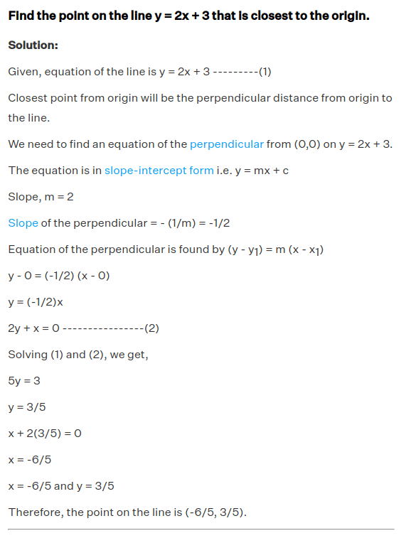
Now, From these infinite solutions, give me a solution that is closest to the origin!
\begin{bmatrix}
3 & 4
\end{bmatrix}
\begin{bmatrix}
x \\ y
\end{bmatrix} = 12
The solution lies on the perpendicular line from the origin? r
Now, From these infinite solutions, give me a solution that is closest to the origin!
\begin{bmatrix}
3 & 4
\end{bmatrix}
\begin{bmatrix}
x \\ y
\end{bmatrix} = 12
The solution lies on the perpendicular line from the origin?
But what is the direction perpendicular to that line?
Now, From these infinite solutions, give me a solution that is closest to the origin!
\begin{bmatrix}
3 & 4
\end{bmatrix}
\begin{bmatrix}
x \\ y
\end{bmatrix} = 12
The solution lies on the perpendicular line from the origin?
But what is the direction perpendicular to that line?
y = -\frac{3}{4}x+3
y=mx+c
m = \frac{\Delta y}{\Delta x}
4
3
\begin{bmatrix}
4 \\ -3
\end{bmatrix}
Now, From these infinite solutions, give me a solution that is closest to the origin!
\begin{bmatrix}
3 & 4
\end{bmatrix}
\begin{bmatrix}
x \\ y
\end{bmatrix} = 12
The solution lies on the perpendicular line from the origin?
But what is the direction perpendicular to that line?
4
3
\begin{bmatrix}
4 \\ -3
\end{bmatrix}
A vector that is perpendicular to [4 3]
\begin{bmatrix}
4\\
-3
\end{bmatrix}
\cdot
v
=
0
v = \begin{bmatrix}
3\\
4
\end{bmatrix}
\begin{bmatrix}
3 \\ 4
\end{bmatrix}
Now, From these infinite solutions, give me a solution that is closest to the origin!
\begin{bmatrix}
3 & 4
\end{bmatrix}
\begin{bmatrix}
x \\ y
\end{bmatrix} = 12
The solution lies on the perpendicular line from the origin?
4
3
\begin{bmatrix}
4 \\ 3
\end{bmatrix}
\begin{bmatrix}
3 \\ 4
\end{bmatrix}
Then This solution is of the form
c \cdot \begin{bmatrix}
3 \\ 4 \end{bmatrix}
Excercise: Find c
Least Norm Solution
Now, From these infinite solutions, give me a solution that is closest to the origin!
Least Norm Solution
\begin{bmatrix}
3 & 4 & 5
\end{bmatrix}
\begin{bmatrix}
x \\ y \\ z
\end{bmatrix} = 12
This is a plane in 3D
Now, From these infinite solutions, give me a solution that is closest to the origin!
Least Norm Solution
\begin{bmatrix}
3 & 4 & 5
\end{bmatrix}
\begin{bmatrix}
x \\ y \\ z
\end{bmatrix} = 12
This is a plane in 3D
Infinite solutions are possible. "Least-Norm" Solution is again in a direction perpendicular to this plane
Direction that is perpendicular to the plane is:
\begin{bmatrix} 3 \\ 4 \\ 5
\end{bmatrix}
Now, From these infinite solutions, give me a solution that is closest to the origin!
\begin{bmatrix}
3 & 4 & 5
\end{bmatrix}
\begin{bmatrix}
x \\ y \\ z
\end{bmatrix} = 12
This is a plane in 3D
Infinite solutions are possible. "Least-Norm" Solution is again in a direction perpendicular to this plane
c \cdot \begin{bmatrix} 3 \\ 4 \\ 5
\end{bmatrix}
Least norm solution is of the form
Now, From these infinite solutions, give me a solution that is closest to the origin!
\begin{bmatrix}
3 & 4 & 5 \\
6 & 7 & 8 \\
\end{bmatrix}
\begin{bmatrix}
x \\ y \\ z
\end{bmatrix} = \begin{bmatrix}
12 \\
13
\end{bmatrix}
What does this mean geometrically?
Now, From these infinite solutions, give me a solution that is closest to the origin!
\begin{bmatrix}
3 & 4 & 5 \\
6 & 7 & 8 \\
\end{bmatrix}
\begin{bmatrix}
x \\ y \\ z
\end{bmatrix} = \begin{bmatrix}
12 \\
13
\end{bmatrix}
What does this mean geometrically?
Intersection of two planes: is a line
Infinite solutions!
Infinite points. Find point, closest to the origin!
The Point is on a line Orthogonal to the Line of intersection of both the planes.
But But, There are Skew lines in 3D!
But it should be on the plane perpendicular to the line
Now, From these infinite solutions, give me a solution that is closest to the origin!
\begin{bmatrix}
3 & 4 & 5 \\
6 & 7 & 8 \\
\end{bmatrix}
\begin{bmatrix}
x \\ y \\ z
\end{bmatrix} = \begin{bmatrix}
12 \\
13
\end{bmatrix}
What does this mean geometrically?
Intersection of two planes: is a line
Infinite solutions!
Infinite points. Find point, closest to the origin!
But But, There are Skew lines in 3D!
But it should be on the plane perpendicular to the line
c_1 \cdot \begin{bmatrix} 3 \\4\\5
\end{bmatrix}
+
c_2 \cdot \begin{bmatrix} 6 \\7\\8
\end{bmatrix}
Now, From these infinite solutions, give me a solution that is closest to the origin!
\begin{bmatrix}
3 & 4 & 5 \\
6 & 7 & 8 \\
\end{bmatrix}
\begin{bmatrix}
x \\ y \\ z
\end{bmatrix} = \begin{bmatrix}
12 \\
13
\end{bmatrix}
Infinite solutions!
c_1 \cdot \begin{bmatrix} 3 \\4\\5
\end{bmatrix}
+
c_2 \cdot \begin{bmatrix} 6 \\7\\8
\end{bmatrix}
LESSON
The least norm solution, always lies in the row space of A
Now, From these infinite solutions, give me a solution that is closest to the origin!
\begin{bmatrix}
3 & 4 & 5 \\
6 & 7 & 8 \\
\end{bmatrix}
\begin{bmatrix}
x \\ y \\ z
\end{bmatrix} = \begin{bmatrix}
12 \\
13
\end{bmatrix}
Infinite solutions!
c_1 \cdot \begin{bmatrix} 3 \\4\\5
\end{bmatrix}
+
c_2 \cdot \begin{bmatrix} 6 \\7\\8
\end{bmatrix}
Theorem
The least norm solution, always lies in the row space of A
Representer Theorem
Ax=b
The least norm solution lies in the rowspace of A. In other words, it is a linear combination of the rows of A
A^Tc
It is of the form
Ax=b
The least norm solution lies in the rowspace of A. In other words, it is a linear combination of the rows of A
A^Tc
It is of the form
A(A^T c) = b
x = (AA^T)^{-1} b
Ax=b
The least norm solution lies in the rowspace of A. In other words, it is a linear combination of the rows of A
A^Tc
It is of the form
A(A^T c) = b
x = (AA^T)^{-1} b
What if AA^T is not invertable????
Resort to Pinv
Pseudoinverse
Pseudoinverse
A = U \Sigma V^T
Column Space
LNS
Row Space
Right Null Space
A is 8x8, with rank 4
Pseudoinverse
A = U \Sigma V^T
Ax=b
Pseudoinverse
A = U \Sigma V^T
Ax=b
(U \Sigma V^T) x=b
U^TU=UU^T = I
U^T(U \Sigma V^T) x= U^T b
Column Space
LNS
Pseudoinverse
A = U \Sigma V^T
Ax=b
(U \Sigma V^T) x=b
U^TU=UU^T = I
U^T(U \Sigma V^T) x= U^T b
Column Space
LNS
Column Space
LNS
B In Col Space
B Not In Col Space
Pseudoinverse
A = U \Sigma V^T
Ax=b
(U \Sigma V^T) x=b
U^TU=UU^T = I
U^T(U \Sigma V^T) x= U^T b
Column Space
LNS
Column Space
LNS
B In Col Space
B Not In Col Space
=
=
Pseudoinverse
A = U \Sigma V^T
Ax=b
(U \Sigma V^T) x=b
U^TU=UU^T = I
I \Sigma V^T x= U^T b
Column Space
LNS
Column Space
LNS
B In Col Space
B Not In Col Space
=
=
Pseudoinverse
A = U \Sigma V^T
Ax=b
(U \Sigma V^T) x=b
U^TU=UU^T = I
\Sigma V^T x= U^T b
\Sigma = \begin{bmatrix}
\sigma_1 & 0 & 0 & \cdots & 0 & 0 & 0 & 0 & 0 \\
0 & \sigma_2 & 0 & \cdots & 0 & 0& 0 & 0 & 0 \\
0 & 0 & \sigma_3 & \cdots & 0 & 0& 0 & 0 & 0 \\
\vdots & \vdots & \ddots & \ddots & \vdots & \vdots & \vdots & \vdots & \vdots \\
0 & \cdots & \cdots & \cdots& \sigma_r & \cdots & 0 & 0 & 0 \\
0 & 0 & 0 & \cdots& \cdots & \cdots & 0 & 0 & 0 \\
0 & 0 & 0 & \cdots& \cdots & \cdots & 0 & 0 & 0 \\
0 & 0 & 0 & \cdots& \cdots & \cdots & 0 & 0 & 0 \\
\end{bmatrix}
\Sigma^{\dagger} = \begin{bmatrix}
\frac{1}{\sigma_1} & 0 & 0 & \cdots & 0 & 0 & 0 & 0 & 0 \\
0 & \frac{1}{\sigma_2} & 0 & \cdots & 0 & 0& 0 & 0 & 0 \\
0 & 0 & \frac{1}{\sigma_3} & \cdots & 0 & 0& 0 & 0 & 0 \\
\vdots & \vdots & \ddots & \ddots & \vdots & \vdots & \vdots & \vdots & \vdots \\
0 & \cdots & \cdots & \cdots& \frac{1}{\sigma_r} & \cdots & 0 & 0 & 0 \\
0 & 0 & 0 & \cdots& \cdots & \cdots & 0 & 0 & 0 \\
0 & 0 & 0 & \cdots& \cdots & \cdots & 0 & 0 & 0 \\
0 & 0 & 0 & \cdots& \cdots & \cdots & 0 & 0 & 0 \\
\end{bmatrix}
Pseudoinverse
A = U \Sigma V^T
Ax=b
(U \Sigma V^T) x=b
U^TU=UU^T = I
V^T x= \Sigma^{\dagger}(U^T b)
\Sigma^{\dagger} = \begin{bmatrix}
\frac{1}{\sigma_1} & 0 & 0 & \cdots & 0 & 0 & 0 & 0 & 0 \\
0 & \frac{1}{\sigma_2} & 0 & \cdots & 0 & 0& 0 & 0 & 0 \\
0 & 0 & \frac{1}{\sigma_3} & \cdots & 0 & 0& 0 & 0 & 0 \\
\vdots & \vdots & \ddots & \ddots & \vdots & \vdots & \vdots & \vdots & \vdots \\
0 & \cdots & \cdots & \cdots& \frac{1}{\sigma_r} & \cdots & 0 & 0 & 0 \\
0 & 0 & 0 & \cdots& \cdots & \cdots & 0 & 0 & 0 \\
0 & 0 & 0 & \cdots& \cdots & \cdots & 0 & 0 & 0 \\
0 & 0 & 0 & \cdots& \cdots & \cdots & 0 & 0 & 0 \\
0 & 0 & 0 & \cdots& \cdots & \cdots & 0 & 0 & 0 \\
\end{bmatrix}
+
+
+
+
+
+
Pseudoinverse
A = U \Sigma V^T
Ax=b
(U \Sigma V^T) x=b
U^TU=UU^T = I
V^T x= \Sigma^{\dagger}(U^T b)
\Sigma^{\dagger} = \begin{bmatrix}
\frac{1}{\sigma_1} & 0 & 0 & \cdots & 0 & 0 & 0 & 0 & 0 \\
0 & \frac{1}{\sigma_2} & 0 & \cdots & 0 & 0& 0 & 0 & 0 \\
0 & 0 & \frac{1}{\sigma_3} & \cdots & 0 & 0& 0 & 0 & 0 \\
\vdots & \vdots & \ddots & \ddots & \vdots & \vdots & \vdots & \vdots & \vdots \\
0 & \cdots & \cdots & \cdots& \frac{1}{\sigma_r} & \cdots & 0 & 0 & 0 \\
0 & 0 & 0 & \cdots& \cdots & \cdots & 0 & 0 & 0 \\
0 & 0 & 0 & \cdots& \cdots & \cdots & 0 & 0 & 0 \\
0 & 0 & 0 & \cdots& \cdots & \cdots & 0 & 0 & 0 \\
0 & 0 & 0 & \cdots& \cdots & \cdots & 0 & 0 & 0 \\
\end{bmatrix}
Pseudoinverse
A = U \Sigma V^T
Ax=b
(U \Sigma V^T) x=b
U^TU=UU^T = I
V^T x= \Sigma^{\dagger}(U^T b)
Row Space
Right Null Space
=
Pseudoinverse
A = U \Sigma V^T
Ax=b
(U \Sigma V^T) x=b
U^TU=UU^T = I
x= V \Sigma^{\dagger}(U^T b)
=
Row Space
Right Null Space
Pseudoinverse
A = U \Sigma V^T
Ax=b
(U \Sigma V^T) x=b
U^TU=UU^T = I
x= V \Sigma^{\dagger}(U^T b)
=
+
+
+
+
+
+
+
+
Pseudoinverse
A = U \Sigma V^T
Ax=b
(U \Sigma V^T) x=b
U^TU=UU^T = I
x= V \Sigma^{\dagger}(U^T b)
=
+
+
+
+
+
+
+
+
Your Solution is a linear combination of Row Space
Pseudoinverse
A = U \Sigma V^T
Ax=b
(U \Sigma V^T) x=b
U^TU=UU^T = I
x= V \Sigma^{\dagger}(U^T b)
=
Pinv Gives: Least Norm Solution
Pseudoinverse
A = U \Sigma V^T
Ax=b
(U \Sigma V^T) x=b
U^TU=UU^T = I
x= V \Sigma^{\dagger}(U^T b)
=
Pinv Gives: Least Norm Solution
If b is not in col space, It gives Least Squares and Least Norm solution
Linear Regression
Linear Regression
y=mx+c
(x_i,y_i)
\begin{bmatrix}
x_1 & 1 \\
x_2 & 1 \\
x_3 & 1 \\
\vdots \\
x_n & 1 \\
\end{bmatrix} \cdot
\begin{bmatrix} m\\ c \end{bmatrix} =
\begin{bmatrix}
y_1\\
y_2 \\
y_3 \\
\vdots \\
y_n \\
\end{bmatrix}
Linear Regression
y=mx+c
(x_i,y_i)
\begin{bmatrix}
x_1 & 1 \\
x_2 & 1 \\
x_3 & 1 \\
\vdots \\
x_n & 1 \\
\end{bmatrix} \cdot
\begin{bmatrix} m\\ c \end{bmatrix} =
\begin{bmatrix}
y_1\\
y_2 \\
y_3 \\
\vdots \\
y_n \\
\end{bmatrix}
\min_w|| y - w^Tx||
\sum_{i=1}^N (y_i - w x_i)^2
X w = Y
Linear Regression
y=mx+c
(x_i,y_i)
\begin{bmatrix}
x_1 & 1 \\
x_2 & 1 \\
x_3 & 1 \\
\vdots \\
x_n & 1 \\
\end{bmatrix} \cdot
\begin{bmatrix} m\\ c \end{bmatrix} \approx
\begin{bmatrix}
y_1\\
y_2 \\
y_3 \\
\vdots \\
y_n \\
\end{bmatrix}
\min_w|| Y - w^T X||_2^2
\sum_{i=1}^N (y_i - w x_i)^2
X w \approx Y
w =X^{\dagger} Y
Kernel Regression
Kernel Regression
Perform Linear Regression, after Mapping Data
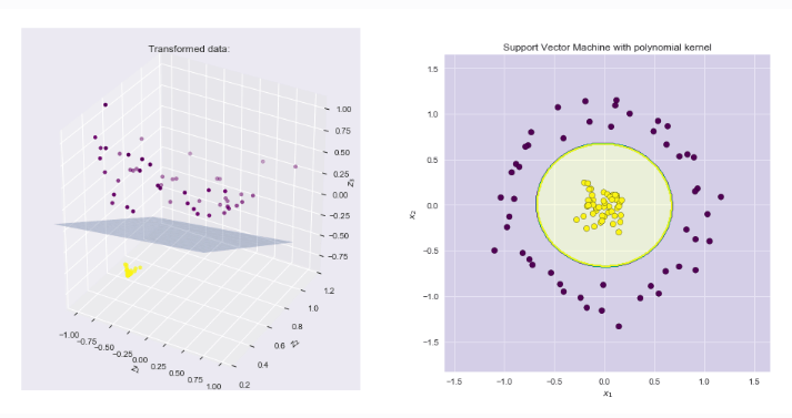
https://xavierbourretsicotte.github.io/Kernel_feature_map.html
Kernel Regression
Perform Linear Regression, after Mapping Data
\psi: \mathbb{R}^d \rightarrow \mathbb{R}^k
L(w) = \sum_{i=1}^N (y_i - w x_i)^2
L(w) = \sum_{i=1}^N (y_i - w \cdot \psi(x_i))^2
Linear Regression
Kernel Regression
Kernel Regression
Perform Linear Regression, after Mapping Data
\psi: \mathbb{R}^d \rightarrow \mathbb{R}^k
L(w) = \sum_{i=1}^N (y_i - w x_i)^2
L(w) = \sum_{i=1}^N (y_i - w \cdot \psi(x_i))^2
Linear Regression
Kernel Regression
Typically we map to higher dimentions, i.e k>d
\mathbb{R}^k
Kernel Regression
Perform Linear Regression, after Mapping Data
\psi: \mathbb{R}^d \rightarrow \mathbb{R}^k
L(w) = \sum_{i=1}^N (y_i - w x_i)^2
L(w) = \sum_{i=1}^N (y_i - w \cdot \psi(x_i))^2
Linear Regression
Kernel Regression
\mathbb{R}^k
We have k unknowns
Kernel Regression
Perform Linear Regression, after Mapping Data
\psi: \mathbb{R}^d \rightarrow \mathbb{R}^k
L(w) = \sum_{i=1}^N (y_i - w \cdot \psi(x_i))^2
Least norm solution,
w = \sum_j^{N} \alpha_j \psi(x_j)
Kernel Regression
\psi: \mathbb{R}^d \rightarrow \mathbb{R}^k
L(\alpha) = \sum_{i=1}^N \left (y_i - \left ( \sum_j^{N} \alpha_j \psi(x_j) \right ) \cdot \psi(x_i) \right)^2
w = \sum_j^{N} \alpha_j \psi(x_j)
\alpha_1 \psi(x_1) \psi(x_i) + \\
\alpha_2 \psi(x_2) \psi(x_i) + \\
\alpha_3 \psi(x_3) \psi(x_i) + \\
\cdots\\
\alpha_n \psi(x_n) \psi(x_i) +
Kernel Regression
\psi: \mathbb{R}^d \rightarrow \mathbb{R}^k
L(w) = \sum_{i=1}^N \left (y_i - \left ( \sum_j^{N} \alpha_j \psi(x_j) \right ) \cdot \psi(x_i) \right)^2
w = \sum_j^{N} \alpha_j \psi(x_j)
\alpha_1 \psi(x_1) \psi(x_i) + \\
\alpha_2 \psi(x_2) \psi(x_i) + \\
\alpha_3 \psi(x_3) \psi(x_i) + \\
\cdots\\
\alpha_n \psi(x_n) \psi(x_i) +
\begin{bmatrix} \alpha_1 & \alpha_2 & \alpha_3 \cdots \alpha_n \end{bmatrix}\begin{bmatrix}
\psi(x_1) \cdot \psi(x_i) \\
\psi(x_2) \cdot \psi(x_i) \\
\psi(x_3) \cdot \psi(x_i) \\
\cdots\\
\psi(x_n) \cdot \psi(x_i)
\end{bmatrix}
Kernel Regression
\psi: \mathbb{R}^d \rightarrow \mathbb{R}^k
L(w) = \sum_{i=1}^N \left (y_i - \left ( \sum_j^{N} \alpha_j \psi(x_j) \right ) \cdot \psi(x_i) \right)^2
w = \sum_j^{N} \alpha_j \psi(x_j)
\begin{bmatrix} \alpha_1 & \alpha_2 & \alpha_3 \cdots \alpha_n \end{bmatrix}\begin{bmatrix}
\psi(x_1) \cdot \psi(x_i) \\
\psi(x_2) \cdot \psi(x_i) \\
\psi(x_3) \cdot \psi(x_i) \\
\cdots\\
\psi(x_n) \cdot \psi(x_i)
\end{bmatrix}
\alpha^T
K(X,x_i)
L(\alpha) = \sum_{i=1}^N \left (y_i - \alpha^T K(X,x_i) \right)^2
Kernel Regression
\psi: \mathbb{R}^d \rightarrow \mathbb{R}^k
L(w) = \sum_{i=1}^N \left (y_i - \left ( \sum_j^{N} \alpha_j \psi(x_j) \right ) \cdot \psi(x_i) \right)^2
w = \sum_j^{N} \alpha_j \psi(x_j)
\begin{bmatrix} \alpha_1 & \alpha_2 & \alpha_3 \cdots \alpha_n \end{bmatrix}\begin{bmatrix}
\psi(x_1) \cdot \psi(x_i) \\
\psi(x_2) \cdot \psi(x_i) \\
\psi(x_3) \cdot \psi(x_i) \\
\cdots\\
\psi(x_n) \cdot \psi(x_i)
\end{bmatrix}
\alpha^T
K(X,x_i)
L(w) = \sum_{i=1}^N \left (y_i - \alpha^T K(X,x_i) \right)^2
N unknowns
Even if we map to "infinite dimensions", we still have to determine only N unknowns
Kernel Regression
\psi: \mathbb{R}^d \rightarrow \mathbb{R}^k
L(w) = \sum_{i=1}^N \left (y_i - \left ( \sum_j^{N} \alpha_j \psi(x_j) \right ) \cdot \psi(x_i) \right)^2
w = \sum_j^{N} \alpha_j \psi(x_j)
L(w) = \sum_{i=1}^N \left (y_i - \alpha^T K(X,x_i) \right)^2
L(w) = || y - \alpha \hat{K} ||_2^2
This is exactly Linear regression over alpha
\hat{K} = \begin{bmatrix}
\psi(x_1) \psi(x_1) & \psi(x_1) \psi(x_2) & \cdots & \psi(x_1) \psi(x_n) \\
\psi(x_2) \psi(x_1) & \psi(x_2) \psi(x_2) & \cdots & \psi(x_2) \psi(x_n) \\
\vdots & \vdots & \ddots & \vdots \\
\psi(x_n) \psi(x_1) & \psi(x_n) \psi(x_n) & \cdots & \psi(x_n) \psi(x_n) \\
\end{bmatrix}
Kernel Regression
\psi: \mathbb{R}^d \rightarrow \mathbb{R}^k
L(w) = \sum_{i=1}^N \left (y_i - \left ( \sum_j^{N} \alpha_j \psi(x_j) \right ) \cdot \psi(x_i) \right)^2
w = \sum_j^{N} \alpha_j \psi(x_j)
L(w) = \sum_{i=1}^N \left (y_i - \alpha^T K(X,x_i) \right)^2
L(w) = || y - \alpha \hat{K} ||_2^2
This is exactly Linear regression over alpha
\alpha \hat{K} = y
\alpha = y \hat{K}^{\dagger}
w = \sum_j^{N} \alpha_j \psi(x_j)
f(x) = y K^{\dagger} K(X,x)
NNGP
Neural Network Gaussian Process
NNGP
Neural Network Gaussian Process
B
A
\phi.
f(x) = A \phi(B \cdot x)
NNGP
Neural Network Gaussian Process
B
A
\phi.
f(x) = A \phi(B \cdot x)
\mathbb{R}^d
\mathbb{R}^{k \times d}
\mathbb{R}^{1 \times k}
k
NNGP
Neural Network Gaussian Process
B
A
\phi.
f(x) = A \phi(B \cdot x)
k
L(w) = \sum_{i=1}^N (y_i - w \cdot A\phi(Bx_i))^2
Mapping x to R^k
B is initialized Randomly
Fix B, Update A only
B_{ij} \sim \mathcal{N}(0,1)
NNGP
Neural Network Gaussian Process
B
A
\phi.
f(x) = A \phi(B \cdot x)
L(w) = \sum_{i=1}^N (y_i - A\phi(Bx_i))^2
Map, do Linear Regression
B_{ij} \sim \mathcal{N}(0,1)
i.e Kernel Regression
L(w) = || y - \alpha \hat{K} ||_2^2
\alpha \hat{K} = y
\alpha = y \hat{K}^{\dagger}
\lim_{k\rightarrow \infty}
A \phi(B \cdot x)
NNGP
Neural Network Gaussian Process
B
A
\phi.
f(x) = \frac{1}{\sqrt{k}} A \phi(B \cdot x)
L(w) = \sum_{i=1}^N (y_i - w \cdot A\phi(Bx_i))^2
Map, do Linear Regression
B_{ij} \sim \mathcal{N}(0,1)
i.e Kernel Regression
L(w) = || y - \alpha \hat{K} ||_2^2
\alpha \hat{K} = y
\alpha = y \hat{K}^{\dagger}
\lim_{k\rightarrow \infty}
A \phi(B \cdot x)
How to calculate the kernel matrix K?
NNGP
Neural Network Gaussian Process
B
A
\phi.
\lim_{k\rightarrow \infty}
How to calculate the kernel matrix K?
L(w) = \sum_{i=1}^N (y_i - A \cdot \frac{1}{\sqrt{k}}\phi(Bx_i))^2
f(x) = \frac{1}{\sqrt{k}} A \phi(B \cdot x)
\hat{K} = \begin{bmatrix}
\psi(x_1) \psi(x_1) & \psi(x_1) \psi(x_2) & \cdots & \psi(x_1) \psi(x_n) \\
\psi(x_2) \psi(x_1) & \psi(x_2) \psi(x_2) & \cdots & \psi(x_2) \psi(x_n) \\
\vdots & \vdots & \ddots & \vdots \\
\psi(x_n) \psi(x_1) & \psi(x_n) \psi(x_n) & \cdots & \psi(x_n) \psi(x_n) \\
\end{bmatrix}
\psi(x) = \frac{1}{\sqrt{k}} \phi(B \cdot x)
K(x,\tilde{x}) = \left \langle \frac{1}{\sqrt{k}} \phi(B \cdot x), \frac{1}{\sqrt{k}} \phi(B \cdot \tilde{x}) \right \rangle
NNGP
Neural Network Gaussian Process
B
A
\phi.
\lim_{k\rightarrow \infty}
How to calculate the kernel matrix K?
L(w) = \sum_{i=1}^N (y_i - A \cdot \frac{1}{\sqrt{k}}\phi(Bx_i))^2
f(x) = \frac{1}{\sqrt{k}} A \phi(B \cdot x)
\psi(x) = \frac{1}{\sqrt{k}} \phi(B \cdot x)
K(x,\tilde{x}) = \left \langle \frac{1}{\sqrt{k}} \phi(B \cdot x), \frac{1}{\sqrt{k}} \phi(B \cdot \tilde{x}) \right \rangle
K(x,\tilde{x}) = \frac{1}{k} \left \langle \phi(B \cdot x), \phi(B \cdot \tilde{x}) \right \rangle
K(x,\tilde{x}) = \frac{1}{k} \sum_i^{k} \phi(B_{i,:} \cdot x ) \cdot \phi(B_{i,:} \cdot \tilde{x})
NNGP
Neural Network Gaussian Process
B
A
\phi.
\lim_{k\rightarrow \infty}
How to calculate the kernel matrix K?
L(w) = \sum_{i=1}^N (y_i - A \cdot \frac{1}{\sqrt{k}}\phi(Bx_i))^2
f(x) = \frac{1}{\sqrt{k}} A \phi(B \cdot x)
\psi(x) = \frac{1}{\sqrt{k}} \phi(B \cdot x)
K(x,\tilde{x}) = \left \langle \frac{1}{\sqrt{k}} \phi(B \cdot x), \frac{1}{\sqrt{k}} \phi(B \cdot \tilde{x}) \right \rangle
K(x,\tilde{x}) = \frac{1}{k} \left \langle \phi(B \cdot x), \phi(B \cdot \tilde{x}) \right \rangle
K(x,\tilde{x}) = \frac{1}{k} \sum_i^{k} \phi(B_{i,:} \cdot x ) \cdot \phi(B_{i,:} \cdot x)
DETOUR: SAMPLING FROM DISTRIBUTIONS AND ESTIMATION OF MEAN
NNGP
Neural Network Gaussian Process
B
A
\phi.
\lim_{k\rightarrow \infty}
How to calculate the kernel matrix K?
f(x) = \frac{1}{\sqrt{k}} A \phi(B \cdot x)
\psi(x) = \frac{1}{\sqrt{k}} \phi(B \cdot x)
K(x,\tilde{x}) = \frac{1}{k} \sum_i^{k} \phi(B_{i,:} \cdot x ) \cdot \phi(B_{i,:} \cdot x)
These are samples from Normal Distributions
We are summing over Samples from "a function of a Random Variable" and taking average
As we take larger and larger k, the more closer estimate of the mean/Expectation we get
NNGP
Neural Network Gaussian Process
B
A
\phi.
\lim_{k\rightarrow \infty}
How to calculate the kernel matrix K?
f(x) = \frac{1}{\sqrt{k}} A \phi(B \cdot x)
\psi(x) = \frac{1}{\sqrt{k}} \phi(B \cdot x)
K(x,\tilde{x}) = \frac{1}{k} \sum_i^{k} \phi(B_{i,:} \cdot x ) \cdot \phi(B_{i,:} \cdot x)
As we take larger and larger k, the more closer estimate of the mean/Expectation we get
w^T
w^T
w \sim \mathcal{N}(0,I)
K(x,\tilde{x}) = \mathop{\mathbb{E}}_{w \sim \mathcal{N}(0,1)} \left [ \phi(w^T x) \phi(w^T \tilde{x}) \right ]
K(x,\tilde{x}) = \mathop{\mathbb{E}}_{w \sim \mathcal{N}(0,1)} \left [ \phi(u) \phi(v) \right ]
NNGP
Neural Network Gaussian Process
B
A
\phi.
\lim_{k\rightarrow \infty}
How to calculate the kernel matrix K?
f(x) = \frac{1}{\sqrt{k}} A \phi(B \cdot x)
\psi(x) = \frac{1}{\sqrt{k}} \phi(B \cdot x)
K(x,\tilde{x}) = \frac{1}{k} \sum_i^{k} \phi(B_{i,:} \cdot x ) \cdot \phi(B_{i,:} \cdot x)
w^T
w^T
K(x,\tilde{x}) = \mathop{\mathbb{E}}_{w \sim \mathcal{N}(0,1)} \left [ \phi(w^T x) \phi(w^T \tilde{x}) \right ]
K(x,\tilde{x}) = \mathop{\mathbb{E}} \left [ \phi(u) \phi(v) \right ]
u and v are from different distributions
u = w^Tx
\mathbb{E}[u] = \mathbb{E}[w_1x_1 + w_2x_2 \cdots w_d x_d]
NNGP
Neural Network Gaussian Process
B
A
\phi.
\lim_{k\rightarrow \infty}
How to calculate the kernel matrix K?
f(x) = \frac{1}{\sqrt{k}} A \phi(B \cdot x)
\psi(x) = \frac{1}{\sqrt{k}} \phi(B \cdot x)
K(x,\tilde{x}) = \frac{1}{k} \sum_i^{k} \phi(B_{i,:} \cdot x ) \cdot \phi(B_{i,:} \cdot x)
w^T
w^T
K(x,\tilde{x}) = \mathop{\mathbb{E}}_{w \sim \mathcal{N}(0,1)} \left [ \phi(w^T x) \phi(w^T \tilde{x}) \right ]
K(x,\tilde{x}) = \mathop{\mathbb{E}} \left [ \phi(u) \phi(v) \right ]
u = w^Tx
\mathbb{E}[u] = \mathbb{E}[w_1x_1 + w_2x_2 \cdots w_d x_d]
\mathbb{E}[u] = \mathbb{E}[w_1x_1 ] + \mathbb{E}[w_2x_2] \cdots \mathbb{E}[w_d x_d] = 0
\mathbb{E}[v] = 0
NNGP
Neural Network Gaussian Process
B
A
\phi.
\lim_{k\rightarrow \infty}
How to calculate the kernel matrix K?
f(x) = \frac{1}{\sqrt{k}} A \phi(B \cdot x)
\psi(x) = \frac{1}{\sqrt{k}} \phi(B \cdot x)
K(x,\tilde{x}) = \frac{1}{k} \sum_i^{k} \phi(B_{i,:} \cdot x ) \cdot \phi(B_{i,:} \cdot x)
w^T
w^T
K(x,\tilde{x}) = \mathop{\mathbb{E}}_{w \sim \mathcal{N}(0,1)} \left [ \phi(w^T x) \phi(w^T \tilde{x}) \right ]
K(x,\tilde{x}) = \mathop{\mathbb{E}} \left [ \phi(u) \phi(v) \right ]
u = w^Tx
\mathbb{E}[v] = 0
\mathbb{E}[u] = 0
Var(u) = Var(w_1x_1 + w_2x_2 \cdots w_d x_d) = x_1^2 Var(w_1) + x_2^2 Var(w_2) \cdots x_d^2 Var(w_d)
Var(u) = x_1^2 + x_2^2 \cdots x_d^2 = ||x||_2^2
cov(u,v) = \langle x, \tilde{x} \rangle
NNGP
Neural Network Gaussian Process
B
A
\phi.
\lim_{k\rightarrow \infty}
How to calculate the kernel matrix K?
f(x) = \frac{1}{\sqrt{k}} A \phi(B \cdot x)
\psi(x) = \frac{1}{\sqrt{k}} \phi(B \cdot x)
K(x,\tilde{x}) = \frac{1}{k} \sum_i^{k} \phi(B_{i,:} \cdot x ) \cdot \phi(B_{i,:} \cdot x)
w^T
w^T
K(x,\tilde{x}) = \mathop{\mathbb{E}}_{w \sim \mathcal{N}(0,1)} \left [ \phi(w^T x) \phi(w^T \tilde{x}) \right ]
K(x,\tilde{x}) = \mathop{\mathbb{E}} \left [ \phi(u) \phi(v) \right ]
\mathbb{E}[v] = 0
\mathbb{E}[u] = 0
Var(u) = ||x||_2^2
Var(v) = ||\tilde{x}||_2^2
cov(u,v) = \langle x,\tilde{x} \rangle
NNGP
Neural Network Gaussian Process
B
A
\phi.
\lim_{k\rightarrow \infty}
How to calculate the kernel matrix K?
f(x) = \frac{1}{\sqrt{k}} A \phi(B \cdot x)
\psi(x) = \frac{1}{\sqrt{k}} \phi(B \cdot x)
K(x,\tilde{x}) = \frac{1}{k} \sum_i^{k} \phi(B_{i,:} \cdot x ) \cdot \phi(B_{i,:} \cdot x)
w^T
w^T
K(x,\tilde{x}) = \mathop{\mathbb{E}}_{w \sim \mathcal{N}(0,1)} \left [ \phi(w^T x) \phi(w^T \tilde{x}) \right ]
K(x,\tilde{x}) = \mathop{\mathbb{E}} \left [ \phi(u) \phi(v) \right ]
u,v \sim \mathcal{N}(0,\Lambda)
\Lambda = \begin{bmatrix}
||x||_2^2 & x \cdot x^T \\
x \cdot x^T & ||\tilde{x}||_2^2
\end{bmatrix}
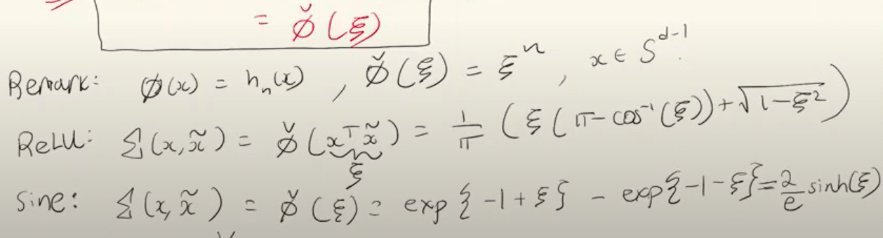
DUAL Activations
\check{\phi}(\epsilon)
NNGP
Neural Network Gaussian Process
B
A
\phi.
\lim_{k\rightarrow \infty}
How to calculate the kernel matrix K?
f(x) = \frac{1}{\sqrt{k}} A \phi(B \cdot x)
\psi(x) = \frac{1}{\sqrt{k}} \phi(B \cdot x)
K(x,\tilde{x}) = \frac{1}{k} \sum_i^{k} \phi(B_{i,:} \cdot x ) \cdot \phi(B_{i,:} \cdot x)
w^T
w^T
K(x,\tilde{x}) = \mathop{\mathbb{E}}_{w \sim \mathcal{N}(0,1)} \left [ \phi(w^T x) \phi(w^T \tilde{x}) \right ]
K(x,\tilde{x}) = \mathop{\mathbb{E}} \left [ \phi(u) \phi(v) \right ]
u,v \sim \mathcal{N}(0,\Lambda)
\Lambda = \begin{bmatrix}
||x||_2^2 & x \cdot x^T \\
x \cdot x^T & ||\tilde{x}||_2^2
\end{bmatrix}
DUAL Activations
\check{\phi}(\epsilon)
\check{\phi}(\epsilon) = \mathop{\mathbb{E}} \left [ \phi(u) \phi(v) \right ]
u,v \sim \mathcal{N}(0,\Lambda)
\Lambda = \begin{bmatrix}
1 & \epsilon\\
\epsilon & 1
\end{bmatrix}
NNGP
Neural Network Gaussian Process
B
A
\phi.
\lim_{k\rightarrow \infty}
How to calculate the kernel matrix K?
f(x) = \frac{1}{\sqrt{k}} A \phi(B \cdot x)
\psi(x) = \frac{1}{\sqrt{k}} \phi(B \cdot x)
K(x,\tilde{x}) = \frac{1}{k} \sum_i^{k} \phi(B_{i,:} \cdot x ) \cdot \phi(B_{i,:} \cdot x)
w^T
w^T
K(x,\tilde{x}) = \mathop{\mathbb{E}}_{w \sim \mathcal{N}(0,1)} \left [ \phi(w^T x) \phi(w^T \tilde{x}) \right ]
K(x,\tilde{x}) = \mathop{\mathbb{E}} \left [ \phi(u) \phi(v) \right ]
u,v \sim \mathcal{N}(0,\Lambda)
\Lambda = \begin{bmatrix}
||x||_2^2 & x \cdot x^T \\
x \cdot x^T & ||\tilde{x}||_2^2
\end{bmatrix}
\check{\phi}(x \tilde{x}^T)
If data is normalized
NNGP
Neural Network Gaussian Process
B
A
\phi.
\lim_{k\rightarrow \infty}
How to calculate the kernel matrix K?
f(x) = \frac{1}{\sqrt{k}} A \phi(B \cdot x)
\psi(x) = \frac{1}{\sqrt{k}} \phi(B \cdot x)
K(x,\tilde{x}) = \frac{1}{k} \sum_i^{k} \phi(B_{i,:} \cdot x ) \cdot \phi(B_{i,:} \cdot x)
w^T
w^T
K(x,\tilde{x}) = \mathop{\mathbb{E}}_{w \sim \mathcal{N}(0,1)} \left [ \phi(w^T x) \phi(w^T \tilde{x}) \right ]
NTK
Neural Tangent Kernel
NTK
f(x) = \frac{1}{\sqrt{k}} A \phi(Bx)
f(w; x) = \frac{1}{\sqrt{k}} A \phi(Bx)
w = \begin{bmatrix}
A_{11} &\cdots & A_{1k} | B_{11} & \cdots B_{kd}
\end{bmatrix}
w \in \mathbb{R}^{k+kd}
NTK
f(x) = \frac{1}{\sqrt{k}} A \phi(Bx)
f(w; x) = \frac{1}{\sqrt{k}} A \phi(Bx)
w = \begin{bmatrix}
A_{11} &\cdots & A_{1k} | B_{11} & \cdots B_{kd}
\end{bmatrix}
"Linearize f around some initialization w"
NTK
f(x) = \frac{1}{\sqrt{k}} A \phi(Bx)
f(w; x) = \frac{1}{\sqrt{k}} A \phi(Bx)
w = \begin{bmatrix}
A_{11} &\cdots & A_{1k} | B_{11} & \cdots B_{kd}
\end{bmatrix}
"Linearize f around some initialization w"
f_x(w) = f_x(w^0) + \nabla f_x(w^0)^T (w-w_0)
NTK
f(x) = \frac{1}{\sqrt{k}} A \phi(Bx)
f(w; x) = \frac{1}{\sqrt{k}} A \phi(Bx)
w = \begin{bmatrix}
A_{11} &\cdots & A_{1k} | B_{11} & \cdots B_{kd}
\end{bmatrix}
"Linearize f around some initialization w"
f_x(w) = f_x(w^0) + \nabla f_x(w^0)^T (w-w_0)
\nabla f_x = \begin{bmatrix}
\frac{\partial f}{\partial A_{11}} \\
\frac{\partial f}{\partial A_{12}} \\
\vdots \\
\frac{\partial f}{\partial B_{kd}} \\
\end{bmatrix}
NTK
f(x) = \frac{1}{\sqrt{k}} A \phi(Bx)
f(w; x) = \frac{1}{\sqrt{k}} A \phi(Bx)
f_x(w) = f_x(w^0) + \nabla f_x(w^0)^T (w-w_0)
Unknown Weights
Can be 0
Then This is a linear model in w
L(w) = \sum_{i=1}^N (y_i - \langle w , \nabla f_{x_i} (w^0)\rangle)^2
NTK
f(x) = \frac{1}{\sqrt{k}} A \phi(Bx)
f(w; x) = \frac{1}{\sqrt{k}} A \phi(Bx)
f_x(w) = f_x(w^0) + \nabla f_x(w^0)^T (w-w_0)
Unknown Weights
Can be 0
Then This is a linear model in w
L(w) = \sum_{i=1}^N (y_i - \langle w , \nabla f_x (w^0)\rangle)^2
This can be intepreted as mapping the data and solving a linear model around w0
NTK
f(x) = \frac{1}{\sqrt{k}} A \phi(Bx)
f(w; x) = \frac{1}{\sqrt{k}} A \phi(Bx)
f_x(w) = f_x(w^0) + \nabla f_x(w^0)^T (w-w_0)
L(w) = \sum_{i=1}^N (y_i - \langle w , \nabla f_x (w^0)\rangle)^2
\phi: x \rightarrow \nabla f_x (w^0)
NTK
f(x) = \frac{1}{\sqrt{k}} A \phi(Bx)
f(w; x) = \frac{1}{\sqrt{k}} A \phi(Bx)
f_x(w) = f_x(w^0) + \nabla f_x(w^0)^T (w-w_0)
L(w) = \sum_{i=1}^N (y_i - \langle w , \nabla f_x (w^0)\rangle)^2
\phi: x \rightarrow \nabla f_x (w^0)
K(x,\tilde{x}) = \langle \nabla f_x(w^0) , \nabla f_{\tilde{x}}(w^0) \rangle
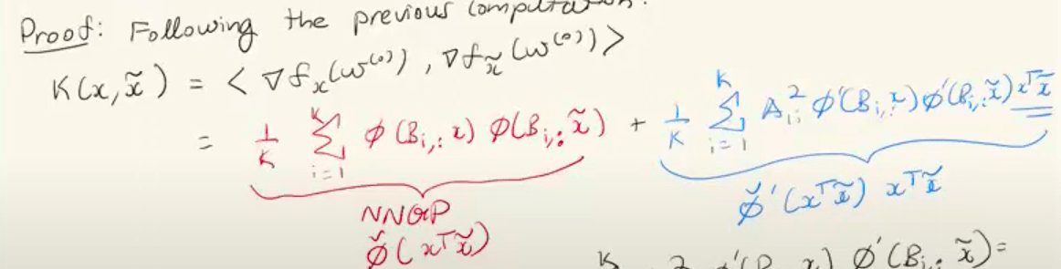
Neural Tangent Kernel
NTK
K(x,\tilde{x}) = \langle \nabla f_x(w^0) , \nabla f_{\tilde{x}}(w^0) \rangle
f(w;x) = A \phi(Bx) = \sum_i^k A_{1i} \phi(B_{i,:} x)
\frac{\partial f}{\partial A_{1i}} = \sum_i \phi(B_{i,:} x)
\frac{\partial f}{\partial B_{ij}} = \sum_i A_{1i} \phi'(B_{i,:} x) x_j
NTK
K(x,\tilde{x}) = \langle \nabla f_x(w^0) , \nabla f_{\tilde{x}}(w^0) \rangle
f(w;x) = A \phi(Bx) = \sum_i^k A_{1i} \phi(B_{i,:} x)
\frac{\partial f}{\partial A_{1i}} = \sum_i \phi(B_{i,:} x)
\frac{\partial f}{\partial B_{ij}} = \sum_i A_{1i} \phi'(B_{i,:} x) x_j
deck
By Incredeble us


