HODMD for Identification of Spatio-Temporal Patterns in Covid19
Standard DMD
v_1
\Delta t
\Delta t
v_2
\Delta t
\Delta t
v_3
\Delta t
\Delta t
\cdots
\cdots
v_K
\Delta t
\Delta t
v_i \in R^J
X_1^K= \begin{bmatrix}
\vdots & \vdots & \cdots & \vdots \\
v_1 & v_2 & \cdots & v_K\\
\vdots & \vdots & \cdots & \vdots
\end{bmatrix}_{J \times K}
J \rightarrow \text{Spatial Dimention}\\
K \rightarrow \text{Temporal Dimention}

Standard DMD
v_1
\Delta t
\Delta t
v_2
\Delta t
\Delta t
v_3
\Delta t
\Delta t
\cdots
\cdots
v_K
\Delta t
\Delta t
v_i \in R^J
X_1^K= \begin{bmatrix}
\vdots & \vdots & \cdots & \vdots \\
v_1 & v_2 & \cdots & v_K\\
\vdots & \vdots & \cdots & \vdots
\end{bmatrix}_{J \times K}
DMD
u_i , a_i , \delta_i , \omega_i
i = 1,2,\cdots M
v_k = \sum_{i=1}^{M} a_i u_i e^{(\delta_i + \omega_i \cdot i) (k-1) \Delta t}
M \rightarrow \text{Spatial Complexity}
dim(span(u_1 , u_2 \cdots u_M))\rightarrow \text{Spectral Complexity}
Standard DMD Reinterpreted: DMD-1 Algorithm
v_1
\Delta t
\Delta t
v_2
\Delta t
\Delta t
v_3
\Delta t
\Delta t
\cdots
\cdots
v_K
\Delta t
\Delta t
v_i \in R^J
X_2^{K} \approx A X_1^{K-1}
Step 1: Dimensionality Reduction
{X}_1^{K-1} \approx U_r \Sigma_r V_r^T
J \times r
r \times r
r \times K
\tilde{X}_1 ^{K-1} = \Sigma_r \cdot V_r^T
r \times r
r \times K
r \times K
{X}_1^{K-1} \approx U_r \tilde{X}_1 ^{K-1}
Rescaled Temporal Modes
Reduced Snapshot Matrix
Standard DMD Reinterpreted: DMD-1 Algorithm
v_1
\Delta t
\Delta t
v_2
\Delta t
\Delta t
v_3
\Delta t
\Delta t
\cdots
\cdots
v_K
\Delta t
\Delta t
v_i \in R^J
X_2^{K} \approx A X_1^{K-1}
Step 1: Dimensionality Reduction
{X}_1^{K-1} \approx U_r \Sigma_r V_r^T
\tilde{X}_1 ^{K-1} \approx \Sigma_r \cdot V_r^T
{X}_1^{K-1} \approx U_r \tilde{X}_1 ^{K-1}
Step 2: Compute DMD Modes and Reduced Koopman Matrix
\tilde{X}_2^{K} \approx \tilde{A} \tilde{X}_1^{K-1}
\tilde{X}_1^{K-1} = U_r \Sigma_r V_r^T
\tilde{A} = X_2^K \cdot (V_r \cdot \Sigma^{-1} \cdot U_r^T)
\tilde{u}_m \rightarrow \text{eigen vectors of } \tilde{A} \\
\mu_m \rightarrow \text{eigen values of } \tilde{A}
u_m = U_r \cdot \tilde{u}_m
\delta_m + i \omega_m = \frac{1}{\Delta t} log(\mu_m)
\tilde{A} \text{ is calculated based on the Koopman Assumption}
X_2^{K} \approx A X_1^{K-1}
Standard DMD Reinterpreted: DMD-1 Algorithm
v_1
\Delta t
\Delta t
v_2
\Delta t
\Delta t
v_3
\Delta t
\Delta t
\cdots
\cdots
v_K
\Delta t
\Delta t
v_i \in R^J
\tilde{A} \text{ is calculated based on the Koopman Assumption}
X_2^{K} \approx A X_1^{K-1}
We Need to Ask the Question, When will the above assumption hold??
Intuitively, There should be Consistency with Spatial Resolution and Temporal Resolution.
This has Direct Effect on the data being "Linear"...
A Balance Between Spatial And Temporal Resolutions should be reached
Standard DMD Reinterpreted: DMD-1 Algorithm
v_1
\Delta t
\Delta t
v_2
\Delta t
\Delta t
v_3
\Delta t
\Delta t
\cdots
\cdots
v_K
\Delta t
\Delta t
v_i \in R^J
\tilde{A} \text{ is calculated based on the Koopman Assumption}
X_2^{K} \approx A X_1^{K-1}
We Need to Ask the Question, When will the above assumption hold??
Should There be a Constraint on Data being Considered? Such that Linearity is Fullfilled?
Standard DMD Reinterpreted: DMD-1 Algorithm
v_1
\Delta t
\Delta t
v_2
\Delta t
\Delta t
v_3
\Delta t
\Delta t
\cdots
\cdots
v_K
\Delta t
\Delta t
v_i \in R^J
X_2^{K} \approx A X_1^{K-1}
Should There be a Constraint on Data being Considered? Such that Linearity is Fullfilled?
Temporal Dimention
Spatial Dimention
Consider One Temporal Dimention
There are 2 points that can be connected by a line
Extending the Argument to higher Dimensions, In general, we might get,
K\leq J
Standard DMD Reinterpreted: DMD-1 Algorithm
v_1
\Delta t
\Delta t
v_2
\Delta t
\Delta t
v_3
\Delta t
\Delta t
\cdots
\cdots
v_K
\Delta t
\Delta t
v_i \in R^J
X_2^{K} \approx A X_1^{K-1}
Linear Consistency
Temporal Dimention
Spatial Dimention
Linearity
X_2^{K} \approx A X_1^{K-1}
[ X_2^{K}, X_1^{K-1} ] \text{ is linear}
null( X_1^{K-1}) \subset null(X_2^{K})
X_2^{K}, X_1^{K-1} \text{ are linearly consistent}
\text{ It can be shown that } X_2^{K} = A X_1^{K-1} \text{ holds Only if they are Linearly Consistent}^*
*Tu, J. H., Rowley, C. W., Luchtenburg, D. M., Brunton, S. L. & Kutz, J. N. On dynamic mode decomposition: Theory and applications. J. Comput. Dyn. 1, 391–421
"nonlinear data is inconsistent and inconsistent data is nonlinear"
\text{ It can be shown that } X_2^{K}, X_1^{K-1} \text{ is Linearly consistent only if its Linear}^*
Standard DMD Reinterpreted: DMD-1 Algorithm
v_1
\Delta t
\Delta t
v_2
\Delta t
\Delta t
v_3
\Delta t
\Delta t
\cdots
\cdots
v_K
\Delta t
\Delta t
v_i \in R^J
X_2^{K} \approx A X_1^{K-1}
Compatiblity Condition (Kim et al.)
Kim et al. : Kim, S., Kim, M., Lee, S. et al. Discovering spatiotemporal patterns of COVID-19 pandemic in South Korea. Sci Rep 11, 24470 (2021). https://doi.org/10.1038/s41598-021-03487-2
K\leq J
"The compatibility condition implies that the linearity of the data T is almost always guaranteed in case m≤n, which then leads to meaningful DMD results. for m>n, T will be in general inconsistent unless it is linear. As such, the direct and reliable DMD analysis of large time series data is not feasible in general." (Kim et al.)
Pitfalls of the DMD-1 Algorithm
Kim et al. : Kim, S., Kim, M., Lee, S. et al. Discovering spatiotemporal patterns of COVID-19 pandemic in South Korea. Sci Rep 11, 24470 (2021). https://doi.org/10.1038/s41598-021-03487-2

Compatable window DMD
Kim et al. : Kim, S., Kim, M., Lee, S. et al. Discovering spatiotemporal patterns of COVID-19 pandemic in South Korea. Sci Rep 11, 24470 (2021). https://doi.org/10.1038/s41598-021-03487-2
CwDMD chooses an adequate set of representative subdomains called windows, each containing a moderate size of time-series data that satisfies the compatibility condition

Kim et. al,
13.6 weeks
10.6 weeks
12.6 weeks
13.3 weeks
K
J = 17
Apply DMD to a subset of dataset which is compatable
K\leq J
Compatable window DMD
Kim et al. : Kim, S., Kim, M., Lee, S. et al. Discovering spatiotemporal patterns of COVID-19 pandemic in South Korea. Sci Rep 11, 24470 (2021). https://doi.org/10.1038/s41598-021-03487-2
CwDMD chooses an adequate set of representative subdomains called windows, each containing a moderate size of time-series data that satisfies the compatibility condition
Kim et. al,
13.6 weeks
10.6 weeks
12.6 weeks
13.3 weeks
K
J = 17
K\leq J

HODMD Motivation
Kim et al. : Kim, S., Kim, M., Lee, S. et al. Discovering spatiotemporal patterns of COVID-19 pandemic in South Korea. Sci Rep 11, 24470 (2021). https://doi.org/10.1038/s41598-021-03487-2
13.6 weeks
10.6 weeks
12.6 weeks
13.3 weeks
K
J = 17
K\leq J
- There is still an upper bound on the temporal resolution.
- Lots of real-world systems possess few spatial points but have rich temporal points.
- There must be a way to circumvent this limitation without compromising on the temporal resolution
- We hence, Propose HODMD as a framework for identifying Spatio-temporal patterns in large time-series.
Developments: On the Effect of Parameter d
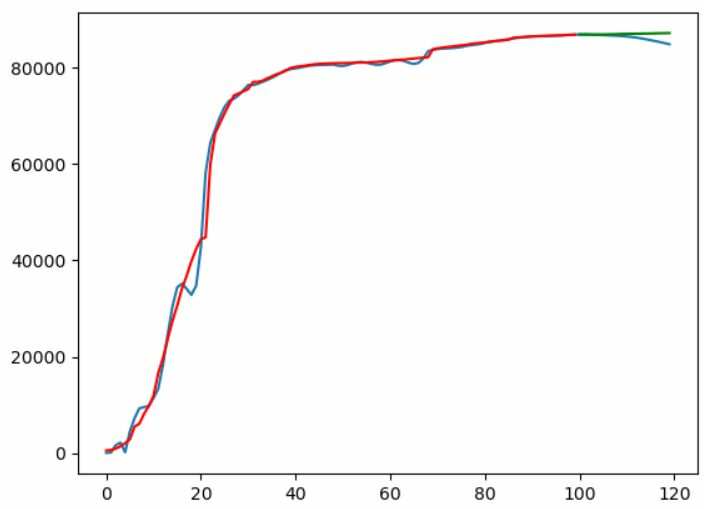
Effect of Parameter d
- It is observed that very less value of d does not aid HODMD
- Similarly, Very high value of D also does ont aid HODMD
Effect of Parameter d
- It is observed that very less value of d does not aid HODMD
- Similarly, Very high value of D also does ont aid HODMD
For a prediction window of 20 days and train days of 40 days, d=20 gave best results
Effect of Parameter d
- It is observed that very less value of d does not aid HODMD
- Similarly, Very high value of D also does ont aid HODMD
For a prediction window of 20 days and train days of 40 days, d=20 gave best results
Further, the literature says that parameter d should be scaled with the same scaling factor that scales the temporal or spatial resolution. [1]
For a prediction window of 20 days and train days of 40 days, d=20 gave best results
Effect of Parameter d
For a prediction window of 20 days and train days of 40 days, d=20 gave best results
The code has been refactored for reproducible research, with increased quality of code.
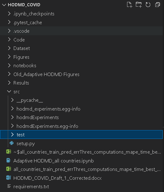
Rigorous Test suite is written to ensure good quality of code
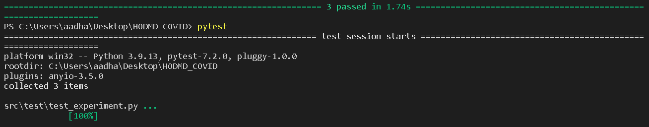
Code is now modular
pip install -e ./src/Install python package (Called hodmdExperiments for now)
from hodmdExperiments.experiment import Experiment
exp = Experiment(covid_data)
exp.fit()
Our experiments hence can be easily reproduced
Developments: Software Engineering perspective: On Enabling Reproducable research
Effect of Parameters
- Train Days
- Pred Days
- parameter-"d"
Interesting Metric:
\xi = \frac{pred\_days \#}{train\_days \#}
We should aim to maximize the above metric
"Get maximum pred_days with minimum train_days"
For a given d, minimizing the below metric will aid our desired results
\frac{1}{\xi} + \sqrt{\frac{1}{N} \sum_i (\hat{y}_i - y_i)^2}
Effect of Parameters
\frac{1}{\xi} + \sqrt{\frac{1}{N} \sum_i (\hat{y}_i - y_i)^2}
Possible Directions.....
Bayesian Optimization for finding parameters, based on the above metric??
Other Possible Directions...
- Different Datasets (We have collected Stock Data and Rainfall Data. Yet to apply HODMD)
- Animations of variations of modes
- Analyze on the effect of parameter d
Other Possible Directions...
- Different Datasets (We have collected Stock Data and Rainfall Data. Yet to apply HODMD)
- Animations of variations of modes
- Analyze on the effect of parameter d
China

0.11753837-0.82817903j
- Real part of Eig Value tells about the growth rate
- Imag part tell about oscillations
JAPAN

0.62842673+0.54379097j
Faster growth Rate than China
India

-0.39535637 -0.70067206j
Text
Why is Re(Eig) negative?????

China
India
BNG
AFG
UK
Detailed Analysis need to be done
Copy of HODMD for Identification of Spatiotemporal Patterns in Covid19
By Incredeble us


