HODMD for Covid19 Cases Forecast and earlywarnings
MIS and SIP Presentation
Team 01
Adaptive HODMD for Forcast of Covid-19 Cases (Theivaprakasham et al.)
Proposed Method
X =
Countries
Text
Days
Train Days
Pred Days
Adaptive HODMD for Forcast of Covid-19 Cases (Theivaprakasham et al.)
Proposed Method
For Each Country,
Countries
Train Days
Pred Days
Days
Train Days
Pred Days
Adaptive HODMD for Forcast of Covid-19 Cases (Theivaprakasham et al.)
Proposed Method
For Each Country,
Countries
Train Days
Pred Days
Days
Train Days
Pred Days
HODMD
d=1
HODMD
d=2
\vdots
d=2
d=len(traindays)
HODMD
Adaptive HODMD for Forcast of Covid-19 Cases (Theivaprakasham et al.)
Proposed Method
For Each Country,
Countries
Train Days
Pred Days
Days
Train Days
Pred Days
HODMD
d=1
HODMD
d=2
\vdots
d=2
d=len(traindays)
HODMD
\phi_i
\lambda_i
\phi_i
\lambda_i
\phi_i
\lambda_i
\phi_i
\lambda_i
\phi_i
\lambda_i
\phi_i
\lambda_i
Pred
Pred
Pred
Error
Error
Error
E\left ( \, \, \, \, , \, \, \, \, \right)
E\left ( \, \, \, \, , \, \, \, \, \right)
E\left ( \, \, \, \, , \, \, \, \, \right)
\hat{E} =
\begin{cases}
E(y,\hat{y}) , if E(y,\hat{y}) \geq E_{threshold} \\
- \infty , if E(y,\hat{y}) \leq E_{threshold}
\end{cases}
d_{min} = \arg \min_{d} \hat{E}(y,\hat{y})
Adaptive HODMD for Forcast of Covid-19 Cases (Theivaprakasham et al.)
Proposed Method
\hat{E} =
\begin{cases}
E(y,\hat{y}) , if E(y,\hat{y}) \geq E_{threshold} \\
- \infty , if E(y,\hat{y}) \leq E_{threshold}
\end{cases}
d_{min} = \arg \min_{d} \hat{E}(y,\hat{y})
Train Days
HODMD
d=1
HODMD
d=2
\vdots
d=2
d=len(traindays)
HODMD
\phi_i
\lambda_i
\phi_i
\lambda_i
\phi_i
\lambda_i
\phi_i
\lambda_i
\phi_i
\lambda_i
\phi_i
\lambda_i
Pred
Pred
Pred
Error
Error
Error
E\left ( \, \, \, \, , \, \, \, \, \right)
E\left ( \, \, \, \, , \, \, \, \, \right)
E\left ( \, \, \, \, , \, \, \, \, \right)
\hat{y} = Y(traindays, len(traindays), len(preddays), E_{threshold}, d)
len(traindays)_{min}, len(preddays)_{min}, d_{min} = \arg \min \hat{E}(y,\hat{y})
Observations
- Error is almost always minimum when training window is large and prediction window is small
- Controlling the error threshold has direct effects on the smoothness of the functions
Adaptive HODMD for Forcast of Covid-19 Cases (Theivaprakasham et al.)
Extentions (By Us)
- Extended Dataset: 203 countries and 1023 points.
- Generated Comparisons with Vannila LSTM and Meta's Prophet (On a subset of dataset)
Adaptive HODMD for Forcast of Covid-19 Cases (Theivaprakasham et al.)
Extentions (By Us): HODMD pred in extended dataset
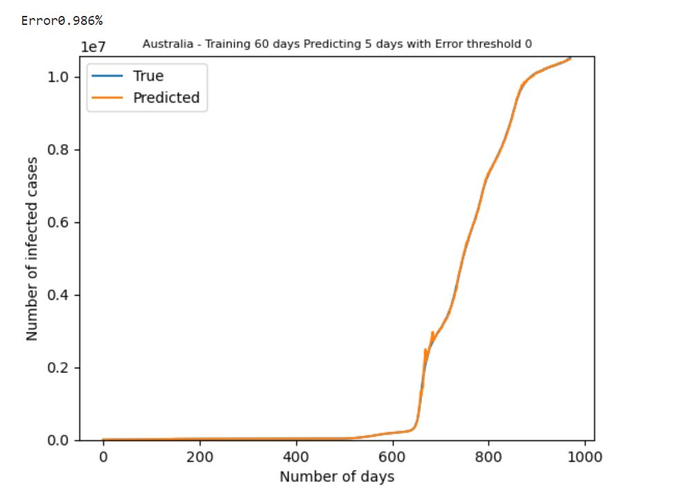


Adaptive HODMD for Forcast of Covid-19 Cases (Theivaprakasham et al.)
Extentions (By Us): Meta's Prophet vs HODMD


Fig: HODMD Prediction
Fig: Meta's Prophet Prediction
First Wave
~150Days
Start of First Wave
Second Wave
~400 Days
Start of Second Wave
Second Wave
~700 Days
Start of Third Wave

VANILLA LSTM: Subject to improvements
HODMD for Identification of Spatio-Temporal Patterns in Covid19
Standard DMD
v_1
\Delta t
\Delta t
v_2
\Delta t
\Delta t
v_3
\Delta t
\Delta t
\cdots
\cdots
v_K
\Delta t
\Delta t
v_i \in R^J
X_1^K= \begin{bmatrix}
\vdots & \vdots & \cdots & \vdots \\
v_1 & v_2 & \cdots & v_K\\
\vdots & \vdots & \cdots & \vdots
\end{bmatrix}_{J \times K}
J \rightarrow \text{Spatial Dimention}\\
K \rightarrow \text{Temporal Dimention}

Standard DMD
v_1
\Delta t
\Delta t
v_2
\Delta t
\Delta t
v_3
\Delta t
\Delta t
\cdots
\cdots
v_K
\Delta t
\Delta t
v_i \in R^J
X_1^K= \begin{bmatrix}
\vdots & \vdots & \cdots & \vdots \\
v_1 & v_2 & \cdots & v_K\\
\vdots & \vdots & \cdots & \vdots
\end{bmatrix}_{J \times K}
DMD
u_i , a_i , \delta_i , \omega_i
i = 1,2,\cdots M
v_k = \sum_{i=1}^{M} a_i u_i e^{(\delta_i + \omega_i \cdot i) (k-1) \Delta t}
M \rightarrow \text{Spatial Complexity}
dim(span(u_1 , u_2 \cdots u_M))\rightarrow \text{Spectral Complexity}
Standard DMD Reinterpreted: DMD-1 Algorithm
v_1
\Delta t
\Delta t
v_2
\Delta t
\Delta t
v_3
\Delta t
\Delta t
\cdots
\cdots
v_K
\Delta t
\Delta t
v_i \in R^J
X_2^{K} \approx A X_1^{K-1}
Step 1: Dimensionality Reduction
{X}_1^{K-1} \approx U_r \Sigma_r V_r^T
J \times r
r \times r
r \times K
\tilde{X}_1 ^{K-1} = \Sigma_r \cdot V_r^T
r \times r
r \times K
r \times K
{X}_1^{K-1} \approx U_r \tilde{X}_1 ^{K-1}
Rescaled Temporal Modes
Reduced Snapshot Matrix
Standard DMD Reinterpreted: DMD-1 Algorithm
v_1
\Delta t
\Delta t
v_2
\Delta t
\Delta t
v_3
\Delta t
\Delta t
\cdots
\cdots
v_K
\Delta t
\Delta t
v_i \in R^J
X_2^{K} \approx A X_1^{K-1}
Step 1: Dimensionality Reduction
{X}_1^{K-1} \approx U_r \Sigma_r V_r^T
\tilde{X}_1 ^{K-1} \approx \Sigma_r \cdot V_r^T
{X}_1^{K-1} \approx U_r \tilde{X}_1 ^{K-1}
Step 2: Compute DMD Modes and Reduced Koopman Matrix
\tilde{X}_2^{K} \approx \tilde{A} \tilde{X}_1^{K-1}
\tilde{X}_1^{K-1} = U_r \Sigma_r V_r^T
\tilde{A} = X_2^K \cdot (V_r \cdot \Sigma^{-1} \cdot U_r^T)
\tilde{u}_m \rightarrow \text{eigen vectors of } \tilde{A} \\
\mu_m \rightarrow \text{eigen values of } \tilde{A}
u_m = U_r \cdot \tilde{u}_m
\delta_m + i \omega_m = \frac{1}{\Delta t} log(\mu_m)
\tilde{A} \text{ is calculated based on the Koopman Assumption}
X_2^{K} \approx A X_1^{K-1}
Standard DMD Reinterpreted: DMD-1 Algorithm
v_1
\Delta t
\Delta t
v_2
\Delta t
\Delta t
v_3
\Delta t
\Delta t
\cdots
\cdots
v_K
\Delta t
\Delta t
v_i \in R^J
\tilde{A} \text{ is calculated based on the Koopman Assumption}
X_2^{K} \approx A X_1^{K-1}
We Need to Ask the Question, When will the above assumption hold??
Intuitively, There should be Consistency with Spatial Resolution and Temporal Resolution.
This has Direct Effect on the data being "Linear"...
A Balance Between Spatial And Temporal Resolutions should be reached
Standard DMD Reinterpreted: DMD-1 Algorithm
v_1
\Delta t
\Delta t
v_2
\Delta t
\Delta t
v_3
\Delta t
\Delta t
\cdots
\cdots
v_K
\Delta t
\Delta t
v_i \in R^J
\tilde{A} \text{ is calculated based on the Koopman Assumption}
X_2^{K} \approx A X_1^{K-1}
We Need to Ask the Question, When will the above assumption hold??
Should There be a Constraint on Data being Considered? Such that Linearity is Fullfilled?
Standard DMD Reinterpreted: DMD-1 Algorithm
v_1
\Delta t
\Delta t
v_2
\Delta t
\Delta t
v_3
\Delta t
\Delta t
\cdots
\cdots
v_K
\Delta t
\Delta t
v_i \in R^J
X_2^{K} \approx A X_1^{K-1}
Should There be a Constraint on Data being Considered? Such that Linearity is Fullfilled?
Temporal Dimention
Spatial Dimention
Consider One Temporal Dimention
There are 2 points that can be connected by a line
Extending the Argument to higher Dimensions, In general, we might get,
K\leq J
Standard DMD Reinterpreted: DMD-1 Algorithm
v_1
\Delta t
\Delta t
v_2
\Delta t
\Delta t
v_3
\Delta t
\Delta t
\cdots
\cdots
v_K
\Delta t
\Delta t
v_i \in R^J
X_2^{K} \approx A X_1^{K-1}
Linear Consistency
Temporal Dimention
Spatial Dimention
Linearity
X_2^{K} \approx A X_1^{K-1}
[ X_2^{K}, X_1^{K-1} ] \text{ is linear}
null( X_1^{K-1}) \subset null(X_2^{K})
X_2^{K}, X_1^{K-1} \text{ are linearly consistent}
\text{ It can be shown that } X_2^{K} = A X_1^{K-1} \text{ holds Only if they are Linearly Consistent}^*
*Tu, J. H., Rowley, C. W., Luchtenburg, D. M., Brunton, S. L. & Kutz, J. N. On dynamic mode decomposition: Theory and applications. J. Comput. Dyn. 1, 391–421
"nonlinear data is inconsistent and inconsistent data is nonlinear"
\text{ It can be shown that } X_2^{K}, X_1^{K-1} \text{ is Linearly consistent only if its Linear}^*
Standard DMD Reinterpreted: DMD-1 Algorithm
v_1
\Delta t
\Delta t
v_2
\Delta t
\Delta t
v_3
\Delta t
\Delta t
\cdots
\cdots
v_K
\Delta t
\Delta t
v_i \in R^J
X_2^{K} \approx A X_1^{K-1}
Compatiblity Condition (Kim et al.)
Kim et al. : Kim, S., Kim, M., Lee, S. et al. Discovering spatiotemporal patterns of COVID-19 pandemic in South Korea. Sci Rep 11, 24470 (2021). https://doi.org/10.1038/s41598-021-03487-2
K\leq J
"The compatibility condition implies that the linearity of the data T is almost always guaranteed in case m≤n, which then leads to meaningful DMD results. for m>n, T will be in general inconsistent unless it is linear. As such, the direct and reliable DMD analysis of large time series data is not feasible in general." (Kim et al.)
Pitfalls of the DMD-1 Algorithm
Kim et al. : Kim, S., Kim, M., Lee, S. et al. Discovering spatiotemporal patterns of COVID-19 pandemic in South Korea. Sci Rep 11, 24470 (2021). https://doi.org/10.1038/s41598-021-03487-2

Compatable window DMD
Kim et al. : Kim, S., Kim, M., Lee, S. et al. Discovering spatiotemporal patterns of COVID-19 pandemic in South Korea. Sci Rep 11, 24470 (2021). https://doi.org/10.1038/s41598-021-03487-2
CwDMD chooses an adequate set of representative subdomains called windows, each containing a moderate size of time-series data that satisfies the compatibility condition

Kim et. al,
13.6 weeks
10.6 weeks
12.6 weeks
13.3 weeks
K
J = 17
Apply DMD to a subset of dataset which is compatable
K\leq J
Compatable window DMD
Kim et al. : Kim, S., Kim, M., Lee, S. et al. Discovering spatiotemporal patterns of COVID-19 pandemic in South Korea. Sci Rep 11, 24470 (2021). https://doi.org/10.1038/s41598-021-03487-2
CwDMD chooses an adequate set of representative subdomains called windows, each containing a moderate size of time-series data that satisfies the compatibility condition
Kim et. al,
13.6 weeks
10.6 weeks
12.6 weeks
13.3 weeks
K
J = 17
K\leq J

HODMD Motivation
Kim et al. : Kim, S., Kim, M., Lee, S. et al. Discovering spatiotemporal patterns of COVID-19 pandemic in South Korea. Sci Rep 11, 24470 (2021). https://doi.org/10.1038/s41598-021-03487-2
13.6 weeks
10.6 weeks
12.6 weeks
13.3 weeks
K
J = 17
K\leq J
- There is still an upper bound on the temporal resolution.
- Lots of real-world systems possess few spatial points but have rich temporal points.
- There must be a way to circumvent this limitation without compromising on the temporal resolution
- We hence, Propose HODMD as a framework for identifying Spatio-temporal patterns in large time-series.
Higher Order DMD
x_{k+1} = A \cdot x_k
- The existence of an operator like A itself is questionable.
- It can be shown that A exists when data is linear....
Higher Order DMD
x_{k+1} = A \cdot x_k
DMD Vs HODMD
DMD Vs HODMD
\begin{bmatrix}
1 \\
1 \\
\end{bmatrix}
\begin{bmatrix}
2 \\
4 \\
\end{bmatrix}
\begin{bmatrix}
3 \\
9 \\
\end{bmatrix}
\begin{bmatrix}
4 \\
16 \\
\end{bmatrix}
\begin{bmatrix}
5\\
25 \\
\end{bmatrix}
Temporal Dimention
Spatial Dimention
Koopman Assumption
x_{k+1} = A x_k
A
A
A
A
Higher Order Koopman Assumption
\begin{bmatrix}
1 \\
1 \\
\end{bmatrix}
\begin{bmatrix}
2 \\
4 \\
\end{bmatrix}
\begin{bmatrix}
3 \\
9 \\
\end{bmatrix}
\begin{bmatrix}
4 \\
16 \\
\end{bmatrix}
\begin{bmatrix}
5\\
25 \\
\end{bmatrix}
Temporal Dimention
Spatial Dimention
R_1
R_2
R_3
R_4
v_{k+d} \approx R_1 v_k + R_2 v_{k+1} \cdots R_d v_{k+d-1}
HODMD
v_{k+d} \approx R_1 v_k + R_2 v_{k+1} \cdots R_d v_{k+d-1}
v_1
\Delta t
\Delta t
v_2
\Delta t
\Delta t
v_3
\Delta t
\Delta t
\cdots
\cdots
v_K
\Delta t
\Delta t
Parameter d can be thought to have weighted "memory" of past d instances of snapshots
DMD-d: HODMD
v_{k+d} \approx R_1 v_k + R_2 v_{k+1} \cdots R_d v_{k+d-1}
v_1
\Delta t
\Delta t
v_2
\Delta t
\Delta t
v_3
\Delta t
\Delta t
\cdots
\cdots
v_K
\Delta t
\Delta t
"Because of this sliding window process, when the spatial complexity N is smaller than the spectral complexity M (very common in nonlinear dynamical systems), DMD-d enables the calculation of several temporal modes associated with a single spatial mode"*
* S.L. Clainche, J.M. Vega, J. Soria, Higher order dynamic mode decomposition of noisy experimental data: the flow structure of a zero-net-mass-flux jet
DMD-d: HODMD
v_{k+d} \approx R_1 v_k + R_2 v_{k+1} \cdots R_d v_{k+d-1}
v_1
\Delta t
\Delta t
v_2
\Delta t
\Delta t
v_3
\Delta t
\Delta t
\cdots
\cdots
v_K
\Delta t
\Delta t
"Because of this sliding window process, when the spatial complexity N is smaller than the spectral complexity M (very common in nonlinear dynamical systems), DMD-d enables the calculation of several temporal modes associated with a single spatial mode. "*
* S.L. Clainche, J.M. Vega, J. Soria, Higher order dynamic mode decomposition of noisy experimental data: the flow structure of a zero-net-mass-flux jet
[1]: Brunton, Steven L., Joshua L. Proctor, and J. Nathan Kutz. "Discovering governing equations from data by sparse identification of nonlinear dynamical systems." Proceedings of the national academy of sciences 113.15 (2016): 3932-3937.
[2]: Takens, Floris. "Detecting strange attractors in turbulence." Dynamical systems and turbulence, Warwick 1980. Springer, Berlin, Heidelberg, 1981. 366-381.
The time-delayed snapshot matrices appearing in Higher-order Koopman Assumption do have something in common with the use of time-delayed snapshots, which has been repeatedly seen to contribute to increasing observability in model 135 identification [1], relying on the Taken’s delay embedding theorem [2].
DMD-d: HODMD
v_{k+d} \approx R_1 v_k + R_2 v_{k+1} \cdots R_d v_{k+d-1}
v_1
\Delta t
\Delta t
v_2
\Delta t
\Delta t
v_3
\Delta t
\Delta t
\cdots
\cdots
v_K
\Delta t
\Delta t
Step 1: Dimensionality Reduction
{X}_1^{K-1} \approx U_r \Sigma_r V_r^T
J \times r
r \times r
r \times K
\tilde{X}_1 ^{K-1} = \Sigma_r \cdot V_r^T
r \times r
r \times K
r \times K
{X}_1^{K-1} \approx U_r \tilde{X}_1 ^{K-1}
Rescaled Temporal Modes
Reduced Snapshot Matrix
DMD-d: HODMD
v_{k+d} \approx R_1 v_k + R_2 v_{k+1} \cdots R_d v_{k+d-1}
v_1
\Delta t
\Delta t
v_2
\Delta t
\Delta t
v_3
\Delta t
\Delta t
\cdots
\cdots
v_K
\Delta t
\Delta t
Step 1: Dimensionality Reduction
{X}_1^{K-1} \approx U_r \Sigma_r V_r^T
\tilde{X}_1 ^{K-1} = \Sigma_r \cdot V_r^T
{X}_1^{K-1} \approx U_r \tilde{X}_1 ^{K-1}
Rescaled Temporal Modes
Reduced Snapshot Matrix
Step 2:
From the Higher-order Koopman Assumption,
\tilde{V}^k_{d+1} \approx \tilde{R_1} \tilde{V}_1^{k-d} + \tilde{R_2} \tilde{V}_1^{k-d+1} + \cdots \tilde{R_d} \tilde{V_d}^{k-1}
\tilde{R}_k \approx U_r^T R_k U_r
\tilde{V}_2^{k-d+1} = \tilde{\bold{R}} \tilde{V}_1^{k-d}

Modified Koopman Matrix
DMD-d: HODMD
v_{k+d} \approx R_1 v_k + R_2 v_{k+1} \cdots R_d v_{k+d-1}
v_1
\Delta t
\Delta t
v_2
\Delta t
\Delta t
v_3
\Delta t
\Delta t
\cdots
\cdots
v_K
\Delta t
\Delta t
Step 1: Dimensionality Reduction
{X}_1^{K-1} \approx U_r \Sigma_r V_r^T
\tilde{X}_1 ^{K-1} = \Sigma_r \cdot V_r^T
{X}_1^{K-1} \approx U_r \tilde{X}_1 ^{K-1}
Rescaled Temporal Modes
Reduced Snapshot Matrix
Step 2:
From the Higher-order Koopman Assumption,
\tilde{V}^k_{d+1} \approx \tilde{R_1} \tilde{V}_1^{k-d} + \tilde{R_2} \tilde{V}_1^{k-d+1} + \cdots \tilde{R_d} \tilde{V_d}^{k-1}
\tilde{R}_k \approx U_r^T R_k U_r
\tilde{V}_2^{k-d+1} = \tilde{\bold{R}} \tilde{V}_1^{k-d}
Reduced Snapshot Matrix
*X variable is V in our explanation(data snapshot)
\tilde{V}_1 ^{k-d+1} = U_r T_1^{k-d+1} , \, T_1^{k-d+1} = \left ( \Sigma_r T_r^T \right)
T_2^{k-d+1} = \bar{R} T_1^{k-d} \,\, , \bar{R} = U_r^T \tilde{R} U_r
\bar{R} = T_2^{k-d+1} \cdot (T_1^{k-d})^{-1}
\text{once } \bar{R} \text{ is known, dynamics can be computed from eigen paris of } \bar{R}
Eigen Values corresponding to countries

-0.39535637+0.70067206j -- Australia
, -0.39535637-0.70067206j, --India
-0.44811384+0.j - Afghanisthan
, 0.98036346+0.03298813j, -- Bangaldesh
0.98036346-0.03298813j, -- Egypt
0.62842673+0.54379097j, -- Japan
0.62842673-0.54379097j, --UAE
0.11753837+0.82817903j, --Spain
0.11753837-0.82817903j --China
Eigen Plot
China

0.11753837-0.82817903j
- Real part of Eig Value tells about the growth rate
- Imag part tell about oscillations
JAPAN

0.62842673+0.54379097j
Faster growth Rate than China
India

-0.39535637 -0.70067206j
Text
Why is Re(Eig) negative?????

China
India
BNG
AFG
UK
Detailed Analysis need to be done
Approach

Data
Data
- Data is collected from Covid-19 India API (COVID19-India API | data (covid19india.org).
- Daywise Data is collected for 38 States and Union Territories.
Data
- Data is collected from Covid-19 India API (COVID19-India API | data (covid19india.org).
- Daywise Data is collected for 38 States and Union Territories.
Bad Data
- NaN Values are "Forwared Filled" , as it is assumed that the next spike in case will be reported. Hence Forward fill sounds like a good way to deal NaN values.
- Rows with negative values are dropped ("UT","DD","UN")
Agumented Data
- Cumulative Sum is taken and cumulative cases with days dataset is constructed. As we would see later this was advantageous for early warnings.
Data Preprocessing
- Exponential Smoothning is applied row-wise, to remove high frequency contents and smooth out the signal
s_t = \alpha \cdot x_t + (1-\alpha) \cdot s_{t-1}
Bayesian Optimization
Bayesian Optimization
Costly, BlackBox
Optimize y
y
inputs
Bayesian Optimization
Hyper-Parameters
TD
D
PD
Bayesian Optimization
Hyper-Parameters
TD
D
PD
Objective
MAE(y,\hat{y}) + \frac{\#TD}{\#PD}
Minimize
Minimum
Maximum
Bayesian Optimization
Hyper-Parameters
TD
D
PD
Objective
MAE(y,\hat{y}) + \frac{\#TD}{\#PD}
Minimize
Minimum
Maximum
The Above Formulation Tells Mathematically that "Give me TD and PD such that, with Minimum TD i will be able to get maximum PD and the model has a reasonable fit"
Bayesian Optimization
Hyper-Parameters
TD
D
PD
Objective
(1-\alpha) \cdot MAE(y,\hat{y}) + \alpha \cdot \frac{\#TD}{\#PD} \\
0 \leq \alpha \leq 1
Minimize
The Above Formulation Tells Mathematically that "Give me TD and PD such that, with Minimum TD i will be able to get maximum PD and the model has a reasonable fit"
Sometimes the model fit is more important than the duration of the prediction. For such scenarios we introduce a term alpha
alpha helps us decide the importance between both the terms
\alpha =0.5
Bayesian Optimization
Hyper-Parameter Optimization: Day Wise
(250 Trials)

Bayesian Optimization
Hyper-Parameter Optimization: Day Wise
(250 Trials)

Text
Bayesian Optimization
Hyper-Parameter Optimization: Choise of HP
(250 Trials)
train_days: 66
pred_days: 18
d: 55
Day Wise Data
train_days: 138
pred_days: 59
d: 99
Cumulative Data
Cumulative Data Gives us more forcast power.
Bayesian Optimization
Hyper-Parameter Optimization: Day Wise
(250 Trials)

Bayesian Optimization
- Based on the initial samples, construct a "surrogate model".
- Upon new data point, calculate the "Expected Improvement"
Bayesian Optimization
- Based on the initial samples, construct a "surrogate model".
- Upon new data point, calculate the "Expected Improvement"
- Acquisition function is used to compute the “EI” metrics in a neighborhood of randomly selected data points, numerically it is maximized with numerical derivative computation
Results


Cumulative Cases vs Days


Early Warning: DayWise (First Wave)
Early Warning: DayWise (Second Wave)

Early Warning: DayWise (Third Wave)

Prediction: 18 days prior
Early Warnings Examples

Able To Predict almost 60 days in Prior
🥳
Absolute Eigen Value Trends

Failed Trials

Failed Trials: Not Interpretable 😔

Thank You
Copy of HODMD for Identification of Spatiotemporal Patterns in Covid19
By Incredeble us


