Statistical learning inference in GW astronomy

He Wang (王赫)

Abtract:

An introduction on model selection of Bayesian inference in GW astronomy (Ref: 1809.02293, book:「Pattern Recognition and Machine Learning」)；
What is KS test and how to plot p-p plot (Ref: 1409.7215)；
(optional) ~~Recent progress of normalized flow in GW data analysis~~ (Ref: 2002.07656/2008.03312 et al.).

Model Selection

According to Bayes theorem, the posterior distribution is given by

p(\theta \mid d)=\frac{\mathcal{L}(d \mid \theta) \pi(\theta)}{\mathcal{Z}}

where \(\mathcal{L}(d \mid \theta)\) is the likelihood function of the data given the \(\theta\),

(where \(\mu(\theta)\) is a template for the gravitational strain waveform given \(\theta\) and \(\sigma\) is the detector noise.)

\(\pi(\theta)\) is the prior distribution of \(\theta\)，

and \(\mathcal{Z}\) is a normalisation factor called the 'evidence', also denote as the fully marginalised likelihood function:

\mathcal{Z} \equiv \int d \theta \mathcal{L}(d \mid \theta) \pi(\theta)

\mathcal{L}(d \mid \theta)=\frac{1}{\sqrt{2 \pi \sigma^{2}}} \exp \left(-\frac{1}{2} \frac{(d-\mu(\theta))^{2}}{\sigma^{2}}\right)

Which model is statistically preferred by the data and by how much?

We wish to distinguish between two hypotheses: \(\mathcal{H}_{0}, \mathcal{H}_{1}\)

\begin{aligned} P\left(\mathcal{H}_{1} \mid d\right) &=\frac{P\left(\mathcal{H}_{1}\right) P\left(d \mid \mathcal{H}_{1}\right)}{P(d)} \\ &=\frac{P\left(\mathcal{H}_{1}\right) P\left(d \mid \mathcal{H}_{1}\right)}{P\left(d \mid \mathcal{H}_{1}\right) P\left(\mathcal{H}_{1}\right)+P\left(d \mid \mathcal{H}_{2}\right) P\left(\mathcal{H}_{2}\right)} \\ &=\frac{\Lambda\left(\mathcal{H}_{1} \mid d\right)}{\Lambda\left(\mathcal{H}_{1} \mid d\right)+P\left(\mathcal{H}_{2}\right) / P\left(\mathcal{H}_{1}\right)} \\ &=\frac{\mathcal{O}\left(\mathcal{H}_{1} \mid d\right)}{\mathcal{O}\left(\mathcal{H}_{1} \mid d\right)+1} \end{aligned}

where we have defined likelihood ratio \(\Lambda\) and odds ratio \(O\):

\begin{aligned} \Lambda\left(\mathcal{H}_{1} \mid d\right) &:=\frac{P\left(d \mid \mathcal{H}_{1}\right)}{P\left(d \mid \mathcal{H}_{0}\right)} \\ \mathcal{O}\left(\mathcal{H}_{1} \mid d\right) &:=\frac{P\left(\mathcal{H}_{1}\right)}{P\left(\mathcal{H}_{0}\right)} \Lambda\left(\mathcal{H}_{1} \mid d\right) = \frac{P\left(\mathcal{H}_{1}\right)}{P\left(\mathcal{H}_{0}\right)} \frac{P\left(d \mid \mathcal{H}_{1}\right)}{P\left(d \mid \mathcal{H}_{0}\right)} \end{aligned}

\mathcal{O}_{B}^{A} \equiv \frac{\mathcal{Z}_{A}}{\mathcal{Z}_{B}} \frac{\pi_{A}}{\pi_{B}} =\frac{\pi_{A}}{\pi_{B}} \mathrm{BF}_{B}^{A}

The odds ratio is the product of the Bayes factor \(\mathrm{BF}_{B}^{A}=\frac{\mathcal{Z}_{A}}{\mathcal{Z}_{B}}\) with the prior odds, which describes our likelihood of hypotheses A and B.

(1809.02293)

Model Selection

Which model is statistically preferred by the data and by how much?

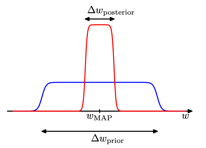
\mathcal{Z} \equiv \int d \theta \mathcal{L}(d \mid \theta) \pi(\theta)

Bayesian evidence encodes two pieces of information:

The likelihood tells us how well our model fits the data.
The act of marginalisation tell us about the size of the volume of parameter space we used to carry out a fit.

(1809.02293)

This creates a sort of tension.

We want to get the best fit possible (high likelihood) but with a minimum prior volume.

A model with a decent fit and a small prior volume often yields a greater evidence than a model with an excellent fit and a huge prior volume.

In these cases, the Bayes factor penalises the more complicated model for being too complicated.

Model Selection

Which model is statistically preferred by the data and by how much?

\mathcal{Z} \equiv \int d \theta \mathcal{L}(d \mid \theta) \pi(\theta)

Bayesian evidence encodes two pieces of information:

The likelihood tells us how well our model fits the data.
The act of marginalisation tell us about the size of the volume of parameter space we used to carry out a fit.

(1809.02293)

This creates a sort of tension.

We want to get the best fit possible (high likelihood) but with a minimum prior volume.

A model with a decent fit and a small prior volume often yields a greater evidence than a model with an excellent fit and a huge prior volume.

In these cases, the Bayes factor penalises the more complicated model for being too complicated.

Some insights into the model evidence by making a simple approximation to the integral over parameters:

Consider first the case of a model having a single parameter w. (M=1)
Assume that the posterior distribution is sharply peaked around the most probable value \(w_\text{MAP}\), with width \(\Delta w_\text{posterior}\).
Assume that the prior is flat with width \(\Delta w_\text{prior}\) so that \(\pi(w) = 1/\Delta w_\text{prior}\).

\mathcal{Z} \equiv \int d w \mathcal{L}(d \mid w) \pi(w) \simeq \mathcal{L}\left(\mathcal{d} \mid w_{\mathrm{MAP}}\right) \frac{\Delta w_{\text {posterior }}}{\Delta w_{\text {prior }}}

\ln \mathcal{Z}(\mathcal{d}) \simeq \ln \mathcal{L}\left(\mathcal{d} \mid w_{\mathrm{MAP}}\right)+M\ln \left(\frac{\Delta w_{\text {posterior }}}{\Delta w_{\text {prior }}}\right)

The first term: the fit to the data given by the most probable parameter values

The second term (Occam factor) penalizes the model according to its complexity

(Pattern Recognition and Machine Learning by C. Bishop)

Model Selection

Which model is statistically preferred by the data and by how much?

\mathcal{Z} \equiv \int d \theta \mathcal{L}(d \mid \theta) \pi(\theta)

Bayesian evidence encodes two pieces of information:

The likelihood tells us how well our model fits the data.
The act of marginalisation tell us about the size of the volume of parameter space we used to carry out a fit.

(1809.02293)

This creates a sort of tension.

We want to get the best fit possible (high likelihood) but with a minimum prior volume.

A model with a decent fit and a small prior volume often yields a greater evidence than a model with an excellent fit and a huge prior volume.

In these cases, the Bayes factor penalises the more complicated model for being too complicated.

\int \mathcal{Z}\left(\mathcal{D} \mid \mathcal{M}_{true}\right) \ln \frac{\mathcal{Z}\left(\mathcal{D} \mid \mathcal{M}_{true}\right)}{\mathcal{Z}\left(\mathcal{D} \mid \mathcal{M}_{1}\right)} \mathrm{d} \mathcal{D}

(1809.02293)

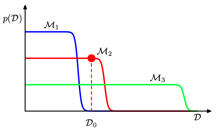
We assume that the true posterior distribution from which the data are considered is contained within the set of models under consideration.

For a given finite data, it is possible for the Bayes factor to be larger for the incorrect model. However, if we average the Bayes factor over the distribution of data sets, we obtain the expected Bayes factor in the form

where the average has been taken with respect to the true distribution of the data. This is an example of Kullback-Leibler divergence.

Comments:

If we compare two models where one model is a superset of the other—for example, we might compare GR and GR with non-tensor modes—and if the data are better explained by the simpler model, the log Bayes factor is typically modest, |log BF| ≈ (1, 2).
It is difficult to completely rule out extensions to existing theories. We just obtain ever tighter constraints on the extended parameter space.
To make good use of Bayesian model comparison, we fully specify priors that are independent of the current data D.
No Occam factors arise in parameter-estimation problems.
On average the Bayes factor will always favour the correct model.

(Pattern Recognition and Machine Learning by C. Bishop)

(Bayesian Astrophysics by A. A. Ramos)

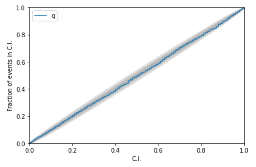
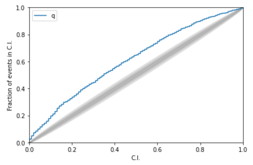
Kolmogorov-Smirnov (KS) Test & Confidence Intervals (C.I.)

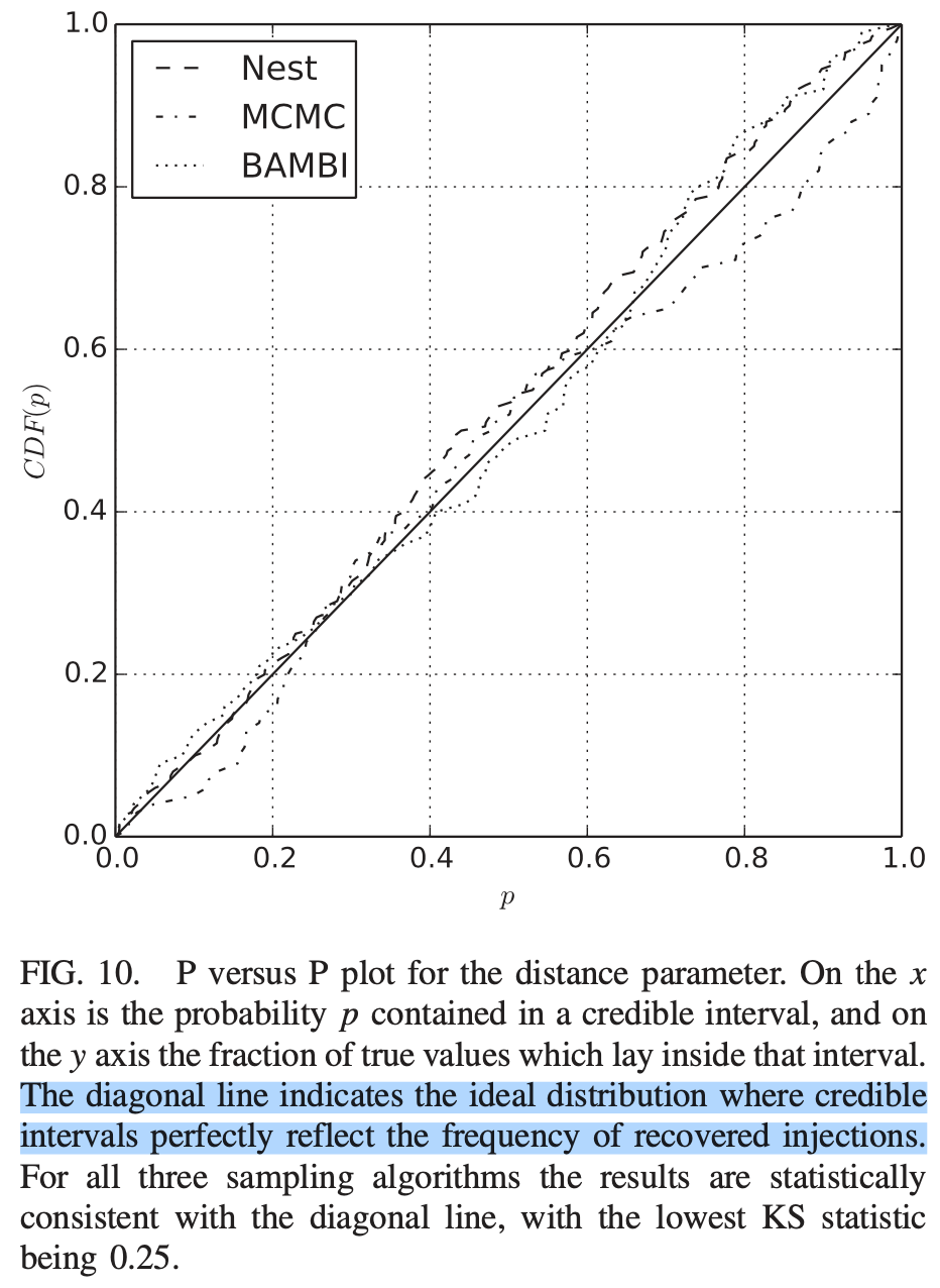
A check to ensure that the probability distributions we recover are truly representative of the confidence we should hold in the parameters of the signal.

By setting up a large set of test injections we can see if this is statistically true by determining the frequency with which the true parameters lie within a certain confidence level.

For each run we calculate credible intervals from the posterior samples, for each parameter. We can then examine the number of times the injected value falls within a given credible interval. If the posterior samples are an unbiased estimate of the true probability, then 10% of the runs should find the injected values within a 10% credible interval, 50% of runs within the 50% interval, and so on.

(1409.7215)

Median-unbiased estimators involve random errors and no systematic errors.

https://en.wikipedia.org/wiki/Bias_of_an_estimator

def pp_plot_scratch(Posterior, TrueParams, 
		x_values = np.linspace(0, 1, 1001)):
    '''
    Posterior - (Num of injections, Num of sampleing)
    TrueParams - (Num of injections, )
    '''
    credible_levels = np.array([sum(pd.Series(Posterior[i]) < T)/len(Posterior[i]) \
    				for i, T in enumerate(TrueParams)])
    pp = np.array([sum(credible_levels < xx) /
                       len(credible_levels) for xx in x_values])
    return pp

Kolmogorov-Smirnov (KS) Test & Confidence Intervals (C.I.)

A check to ensure that the probability distributions we recover are truly representative of the confidence we should hold in the parameters of the signal.

x_{poster}\sim \mathcal{N} [\mathcal{N}(x_{true}, \sigma_\mu) , \sigma_{poster}]

\sigma_\mu = \sigma_{poster}

\sigma_\mu > \sigma_{poster}

\sigma_\mu < \sigma_{poster}

A test for pp-plot:

Kolmogorov-Smirnov (KS) Test & Confidence Intervals (C.I.)

A check to ensure that the probability distributions we recover are truly representative of the confidence we should hold in the parameters of the signal.

A test for pp-plot:

x_{poster}\sim \mathcal{N} [\mathcal{N}(x_{true}+\epsilon, \sigma_\mu) , \sigma_{poster}]

\sigma_\mu = \sigma_{poster}

\sigma_\mu > \sigma_{poster}

\sigma_\mu < \sigma_{poster}

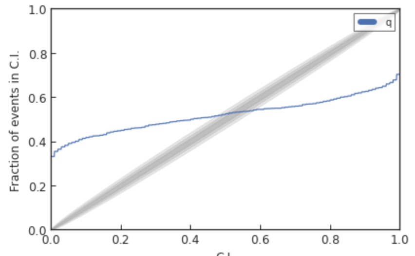
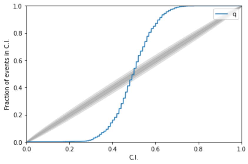
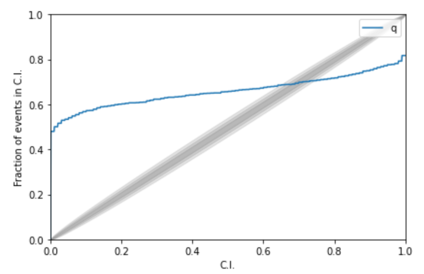
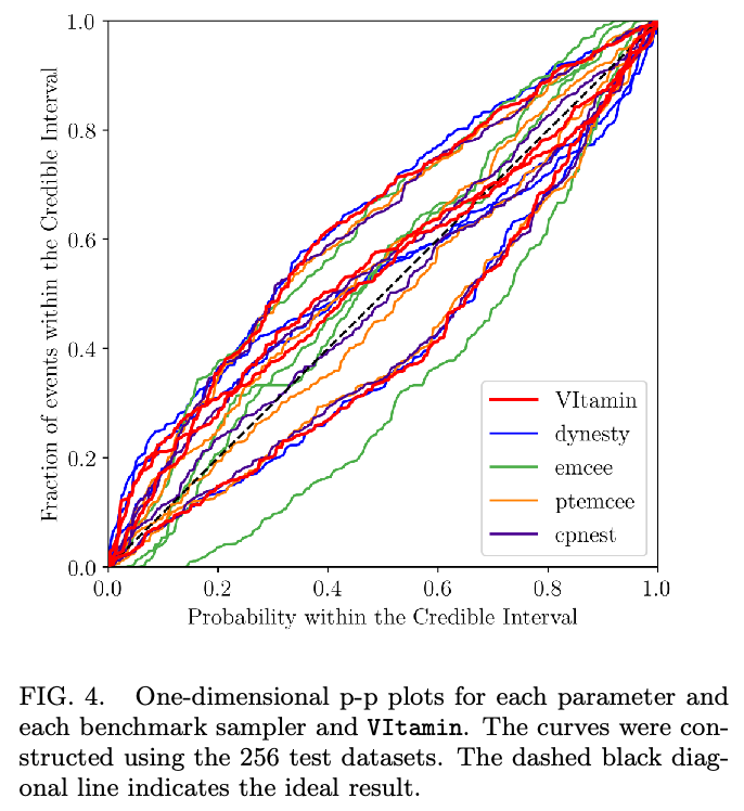
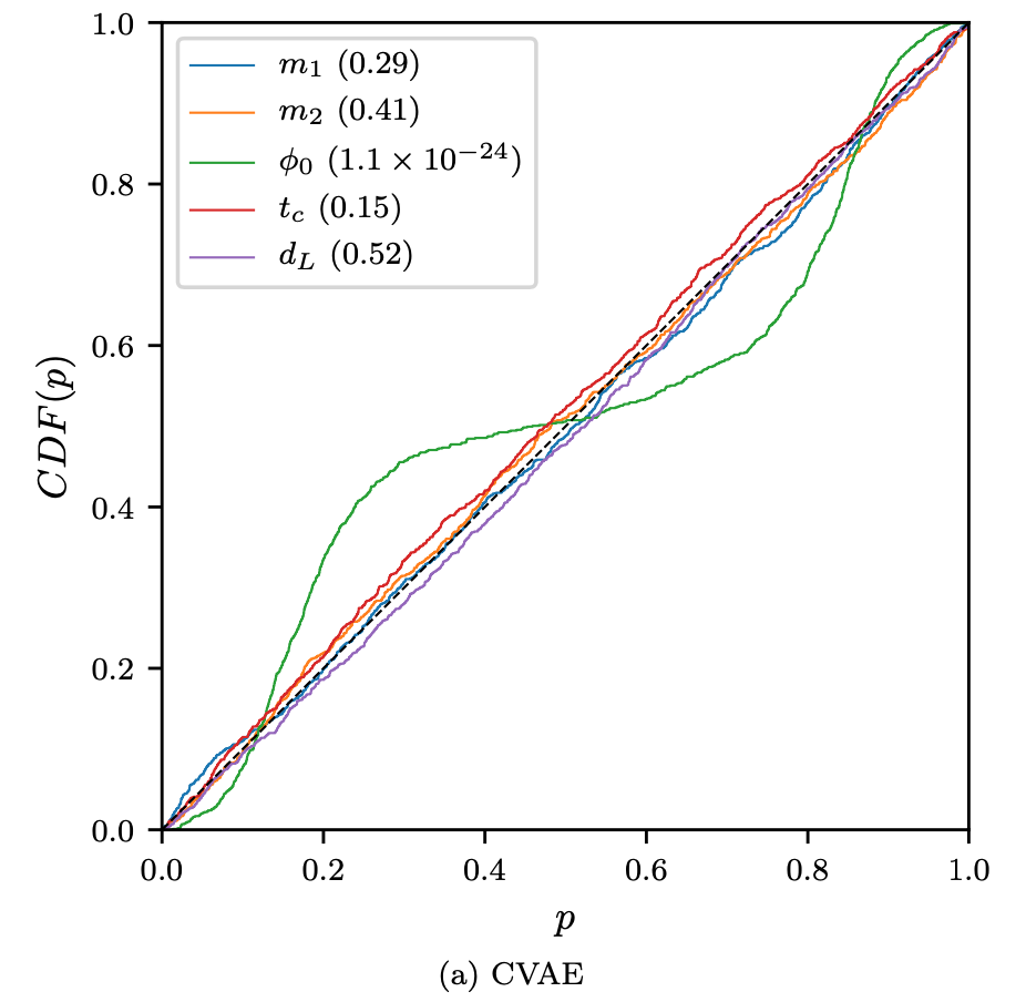
Kolmogorov-Smirnov (KS) Test & Confidence Intervals (C.I.)

A check to ensure that the probability distributions we recover are truly representative of the confidence we should hold in the parameters of the signal.

Some cases:

(2008.03312)

(2002.07656)

(1909.06296)

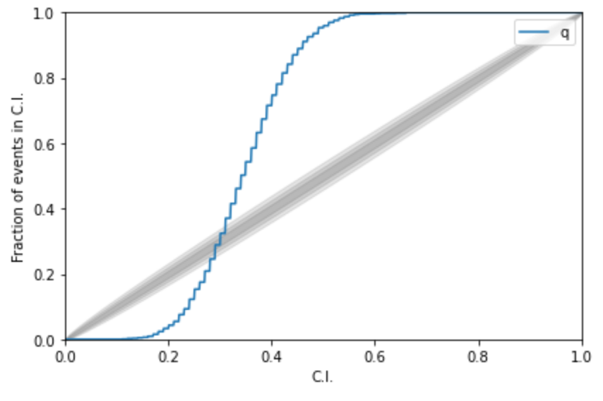
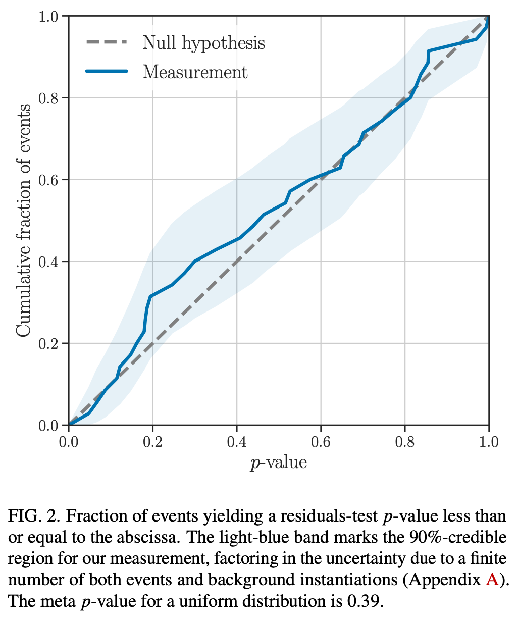
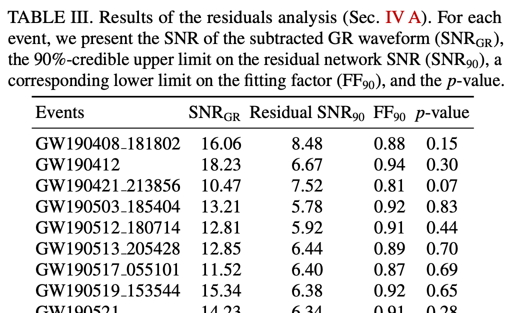
Kolmogorov-Smirnov (KS) Test & Confidence Intervals (C.I.)

A check to ensure that the probability distributions we recover are truly representative of the confidence we should hold in the parameters of the signal.

Some cases:

(TGR for GWTC2 from LSC)

To evaluate whether the Residual value (90%-credible upper-limit), \(\text{SNR}_{90}\), is consistent with instrumental noise fluctuations...
we measure the coherent power in ~200 sets of noise-only detector data around each event.
This yields a p-value for noise-producing coherent power with \(\text{SNR}^n_{90}\) greater than or equal to the residual value \(\text{SNR}_{90}\), i.e., \(p=P\left(\mathrm{SNR}_{90}^{\mathrm{n}} \geq\right. \text { SNR }_{90} \text { | noise) }\)
If the set of p-values is consistent with all coherent residual power being due to instrumental noise, we expect the p-values to be uniformly distributed over [0, 1].
This demonstrates no statistically significant deviations between the observed residual power and the detector noise around the set of events.

Statistical learning inference in GW astronomy

By He Wang

Statistical learning inference in GW astronomy

Abtract: 1. An introduction on model selection of Bayesian inference in GW astronomy (Ref: 1809.02293, book:「Pattern Recognition and Machine Learning」)；2. What is KS test and how to plot p-p plot (Ref: 1409.7215)；3. (optional) Recent progress of normalized flow in GW data analysis (Ref: 2002.07656/2008.03312 et al.).

He Wang PRO

Knowledge increases by sharing but not by saving.

Statistical learning inference in GW astronomy

More from He Wang