
























He Wang PRO
Knowledge increases by sharing but not by saving.
Aug 2, NZ Gravity seminar @UoA
He Wang (王赫)
hewang@ucas.ac.cn
International Centre for Theoretical Physics Asia-Pacific (ICTP-AP), UCAS
Taiji Laboratory for Gravitational Wave Universe (Beijing/Hangzhou), UCAS
On behalf of the LIGO-VIRGO-KAGRA collaborations
In 1916, A. Einstein proposed the GR and predicted the existence of GW.
Gravitational waves (GW) are a strong field effect in the GR.
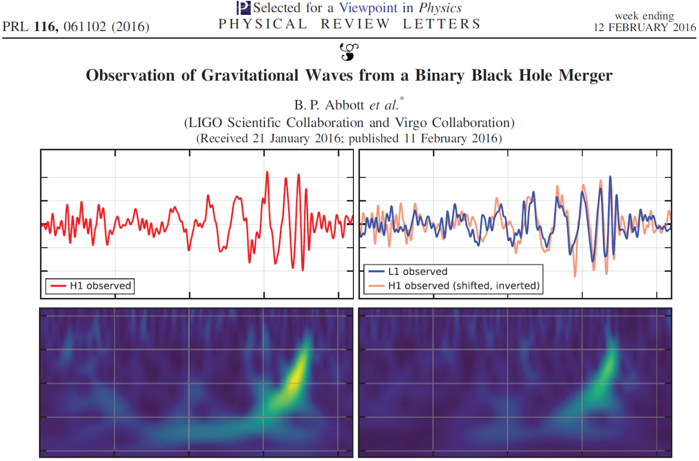
2015: the first experimental detection of GW from the merger of two black holes was achieved.
2017: the first multi-messenger detection of a BNS signal was achieved, marking the beginning of multi-messenger astronomy.
2017: the Nobel Prize in Physics was awarded for the detection of GW.
As of now: more than 90 gravitational wave events have been discovered.
O4, which began on May 24th 2023, is currently in progress.
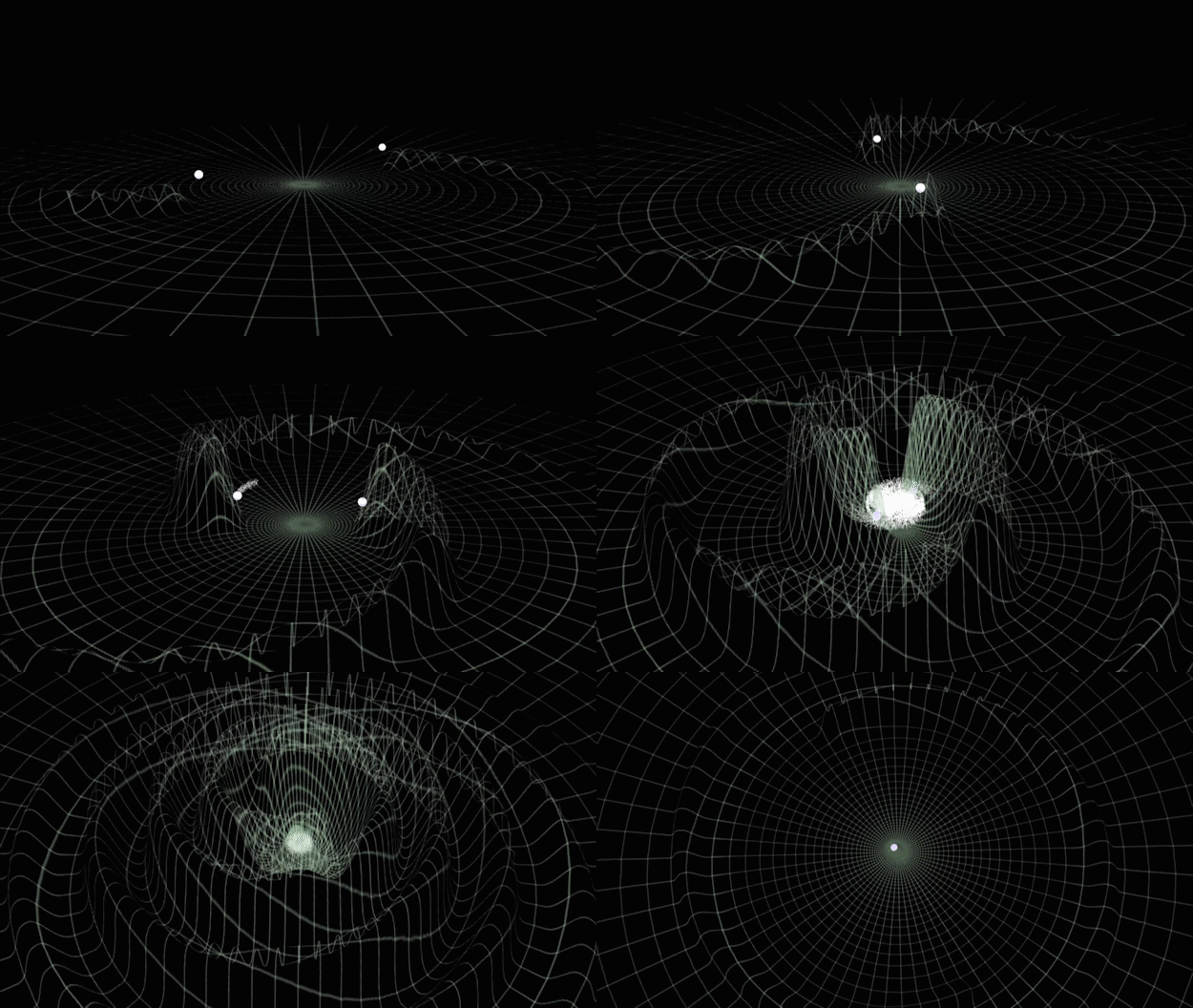
Gravitational waves generated by binary black holes system
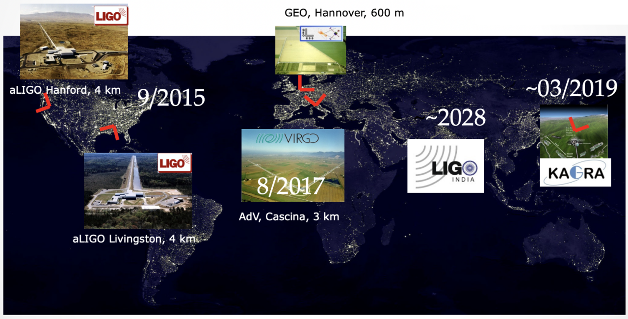
GW detector
LIGO-VIRGO-KAGRA network
2017 Nobel Prize in Physics
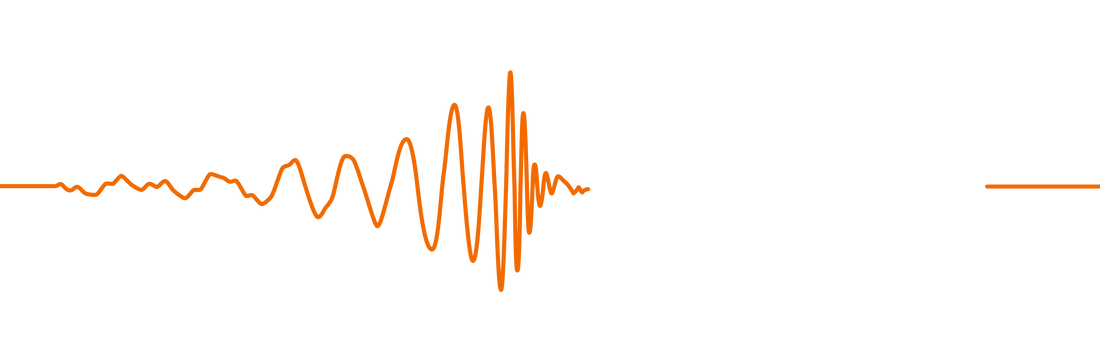
The first GW event of GW150914
—— Bernard F. Schutz
DOI: 10.1063/1.1629411
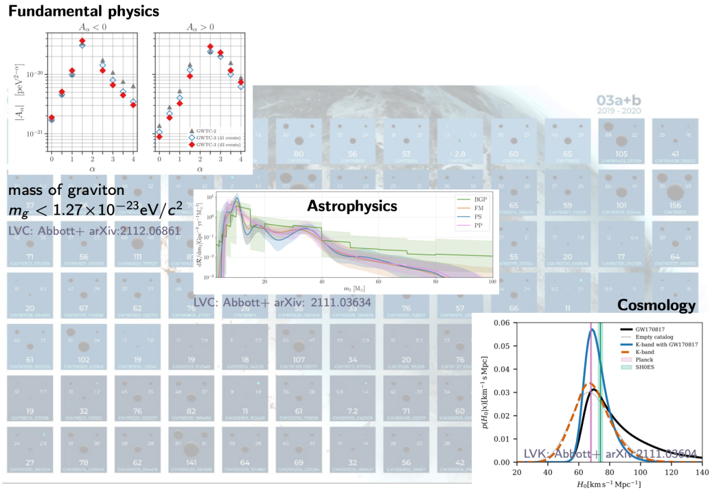
GWTC-3
GW Data characteristics
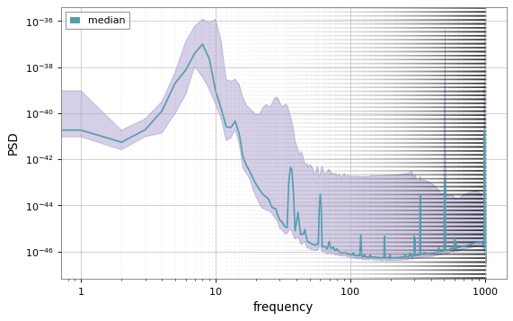
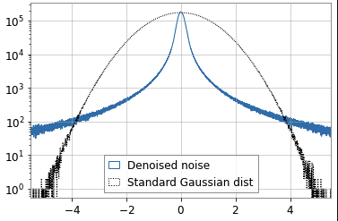
Noise: non-Gaussian and non-stationary
Signal:
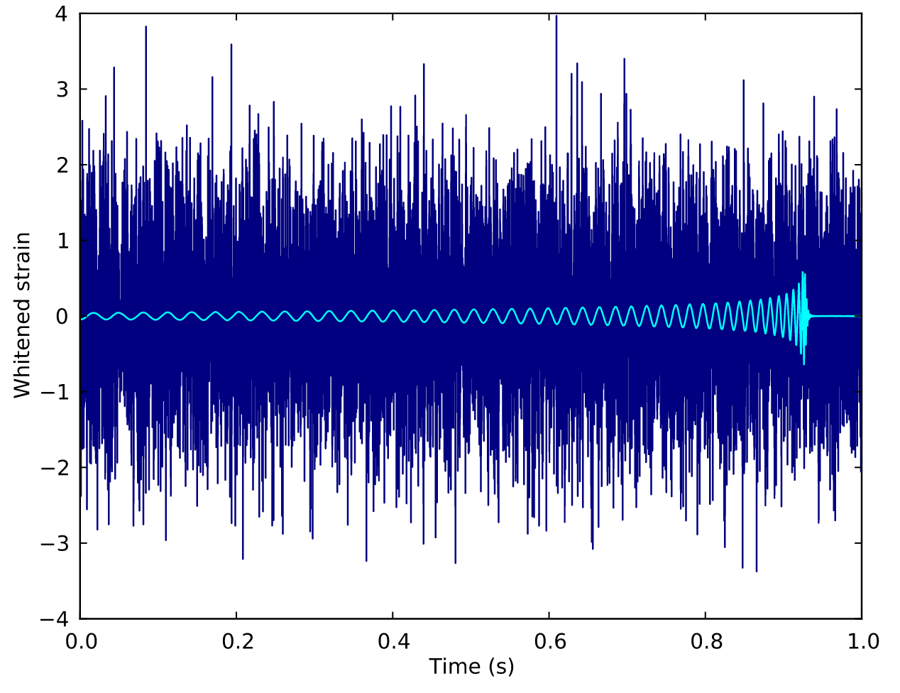
(Earth-based) A low signal-to-noise ratio (SNR) which is typically about 1/100 of the noise amplitude (-60 dB).
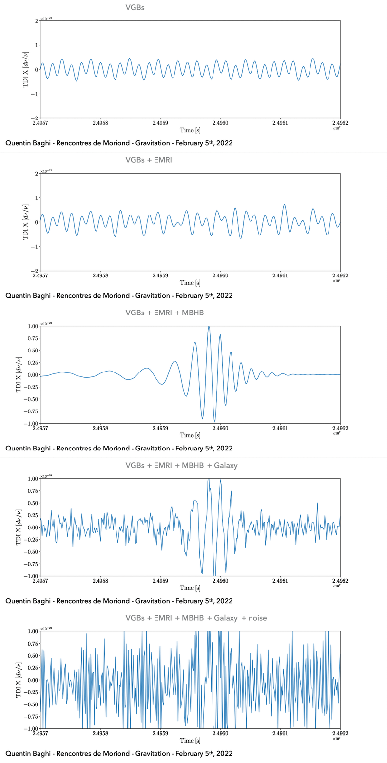
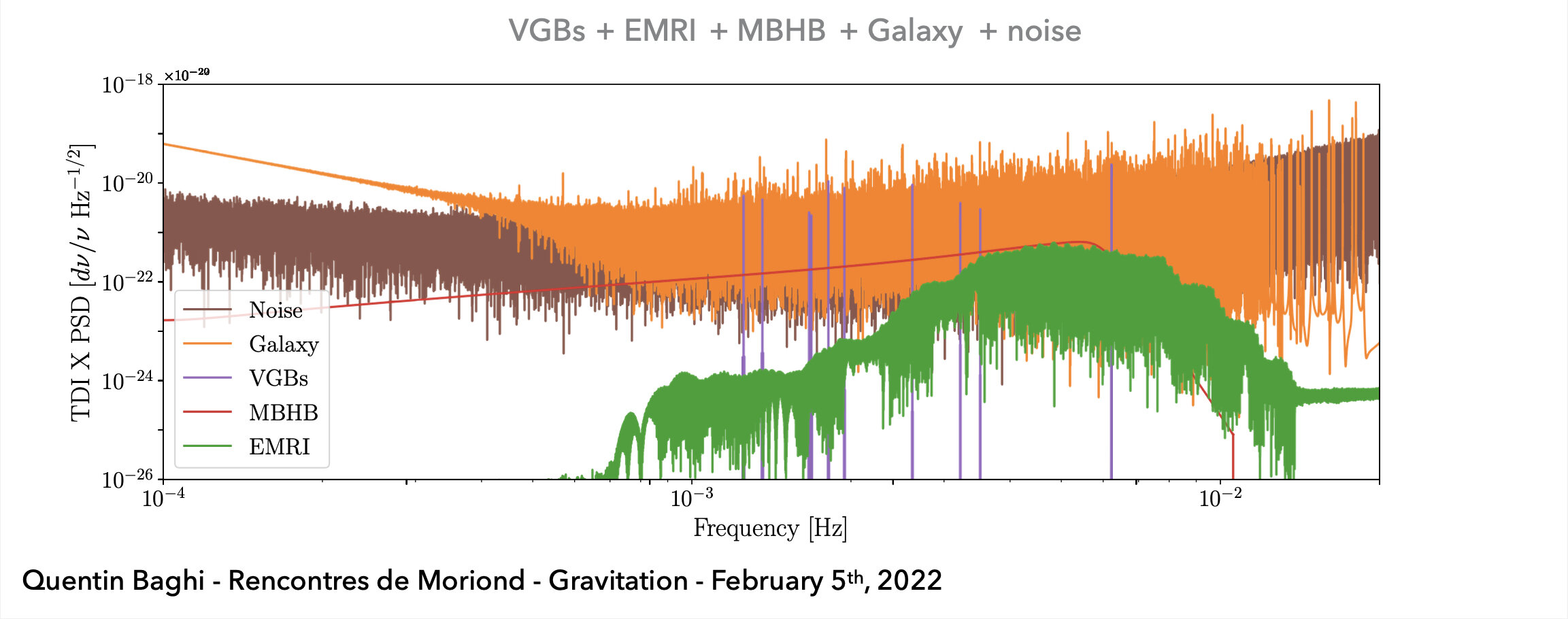
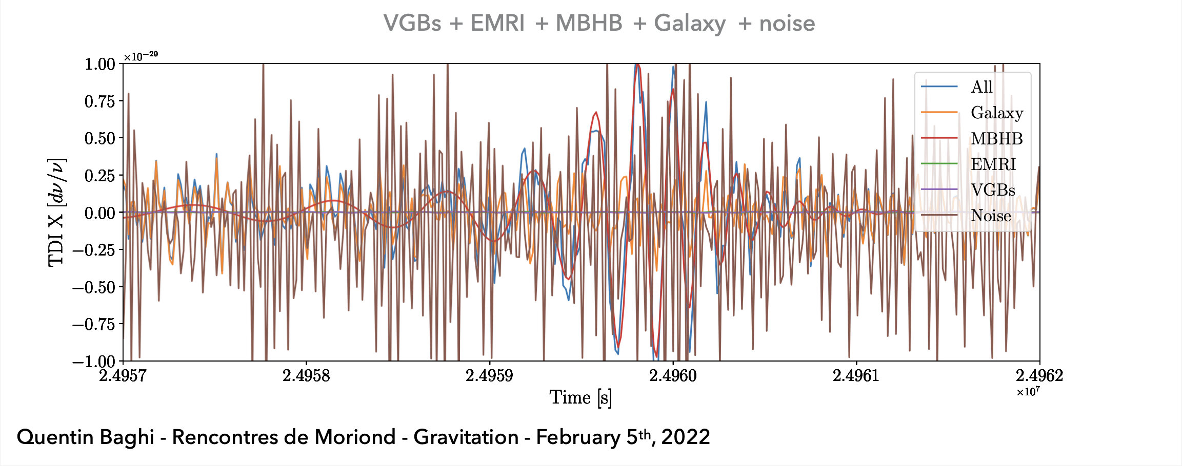
(Space-based) A superposition of all GW signals (e.g.: \(10^4\) of GBs, \(10\sim10^2\) of SMBHs, and \(10\sim10^3\) of EMRIs, etc.) received during the mission's observational run.
Matched filtering techniques
In Gaussian and stationary noise environments, the optimal linear algorithm for extracting weak signals
LIGO-VIRGO-KAGRA
LISA / Taiji project
Frequentist hypothesis testing and likelihood princple:
make some assumptions about signal and noise hypothesis
write down the likelihood function for a signal in noise
find the parameters that maximise it
define a corresponding detection statistic
\(\rightarrow\) recover the MFPioneering works utilizing CNN
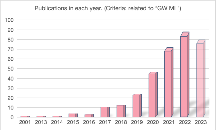
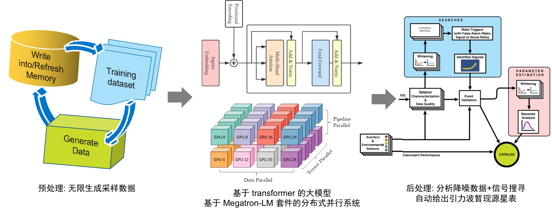
AI for Science \(\rightarrow\) AI for GW Astronomy
Exported: Oct, 2023 (in preparation)
PRL, 2018, 120(14): 141103.
PRD, 2018, 97(4): 044039.
Matched-filtering Convolutional Neural Network (MFCNN)
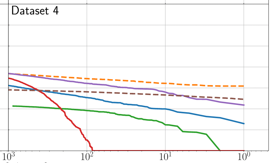
MLGWSC-1
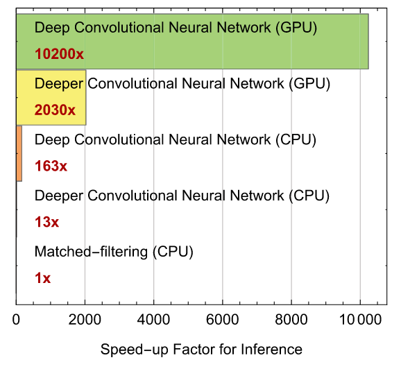
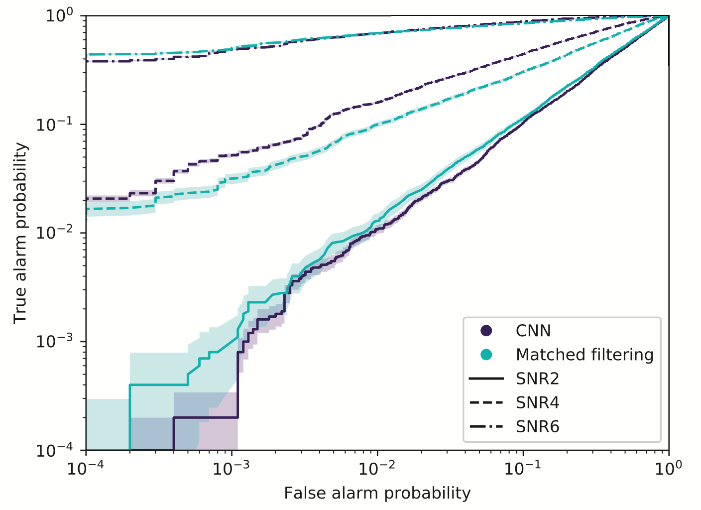
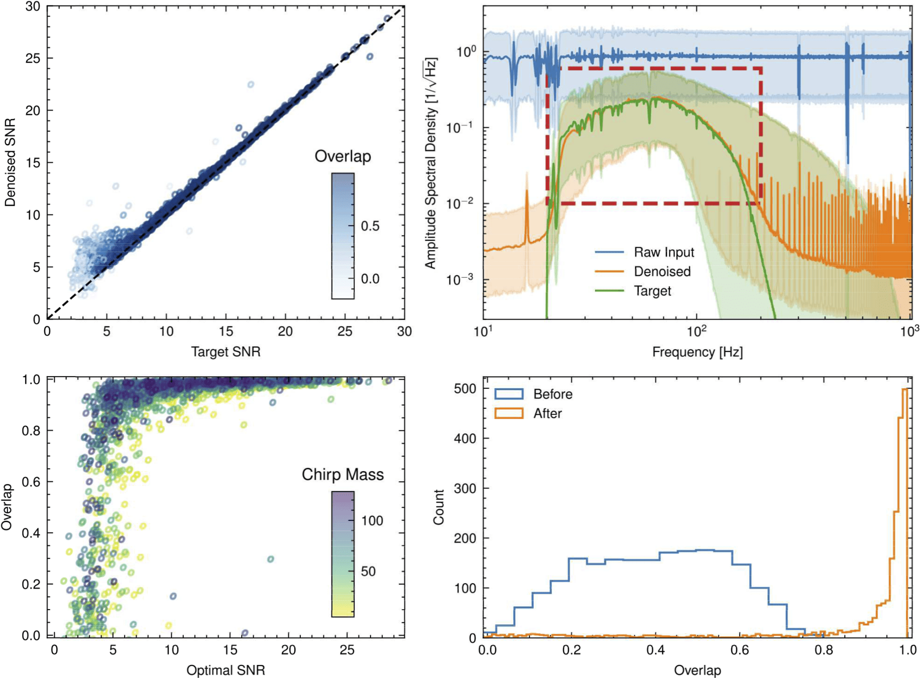
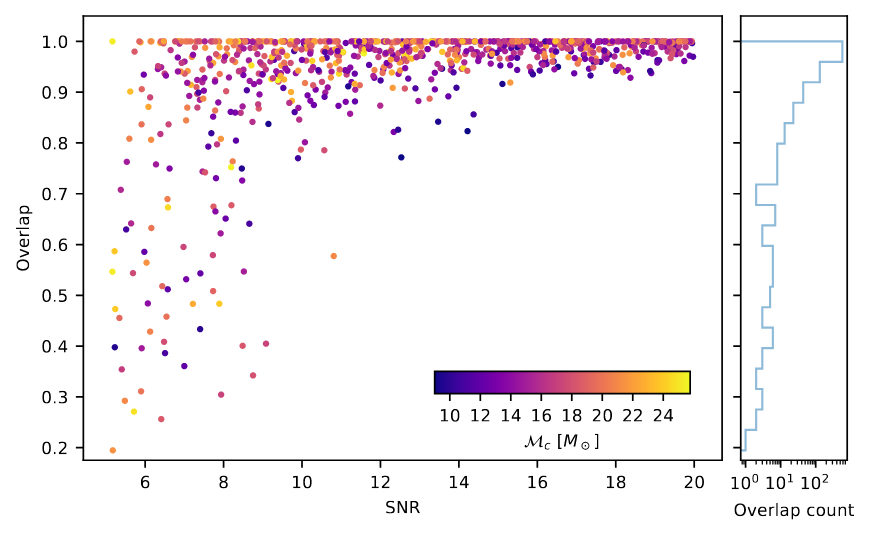
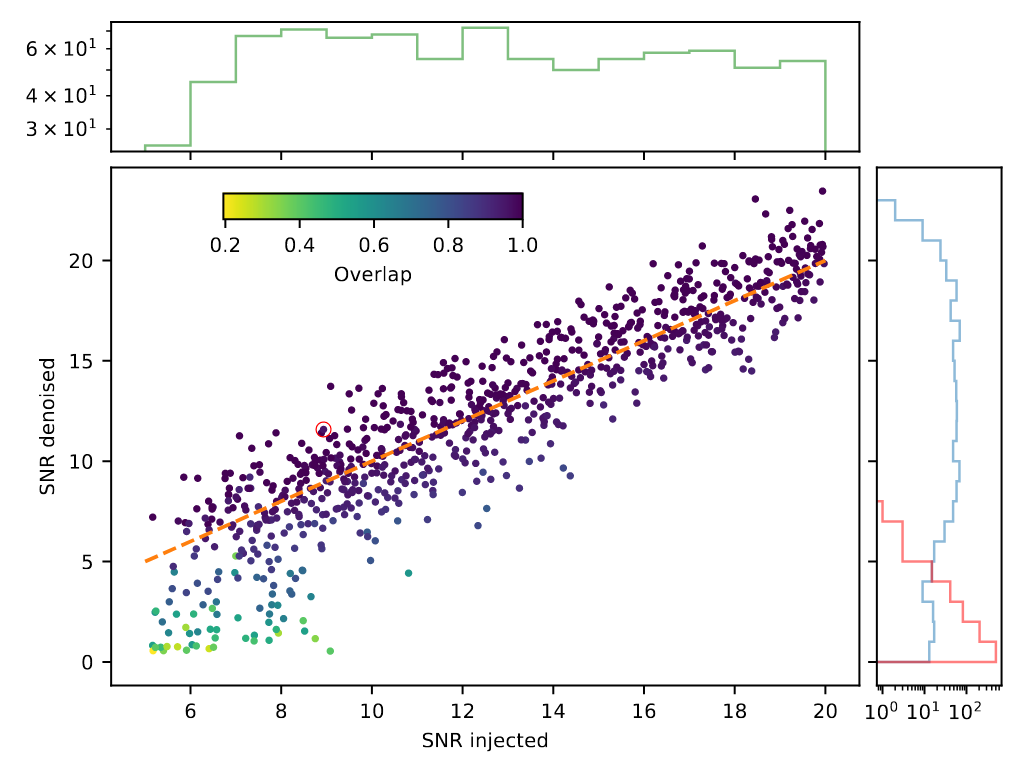
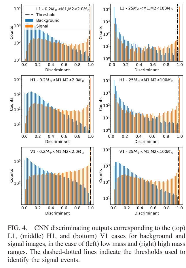
The majority of AI algorithms used for testing are highly sensitive to non-Gaussian real noise backgrounds, resulting in high false positive rates.
(MFCNN group) H.W., et al. PRD (2023)
CL.M., W.W., H.W., et al. PRD (2022)
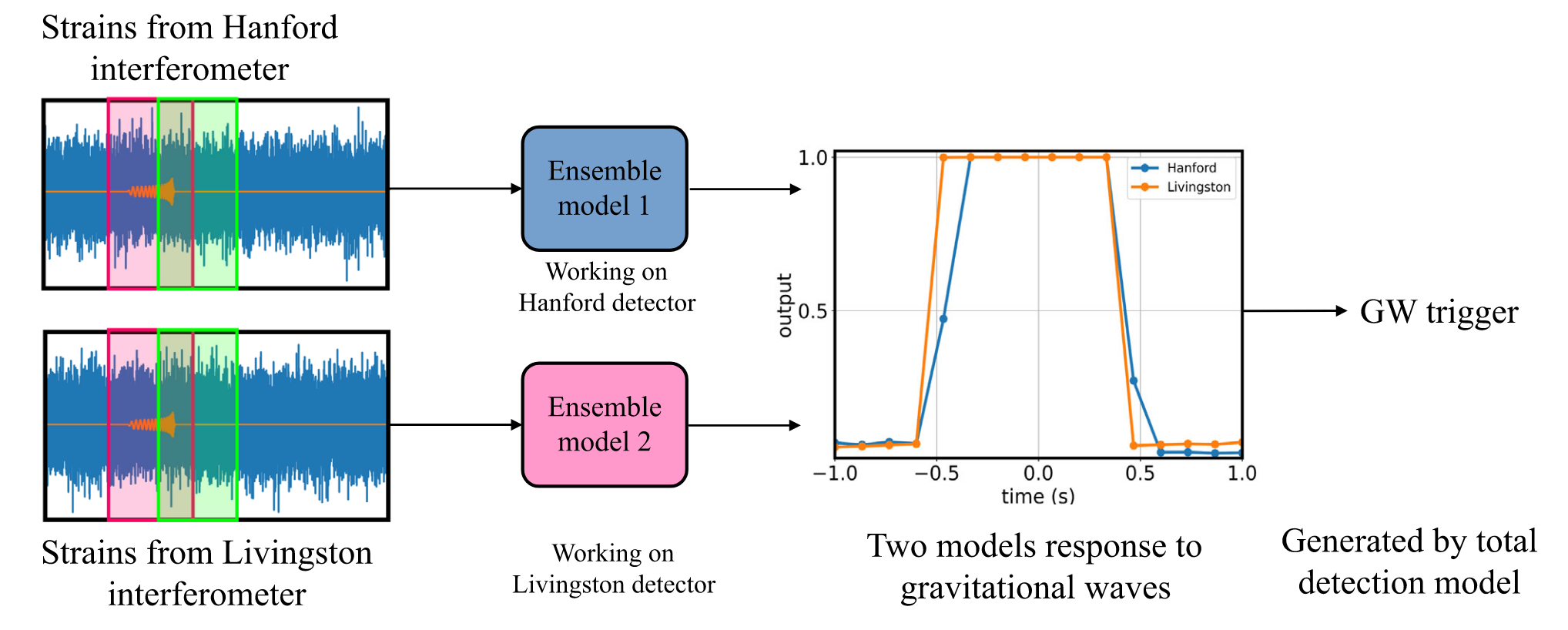
Ensemble learning
Leverages statistical approaches to utilize more information for making informed decisions by combining multiple models.
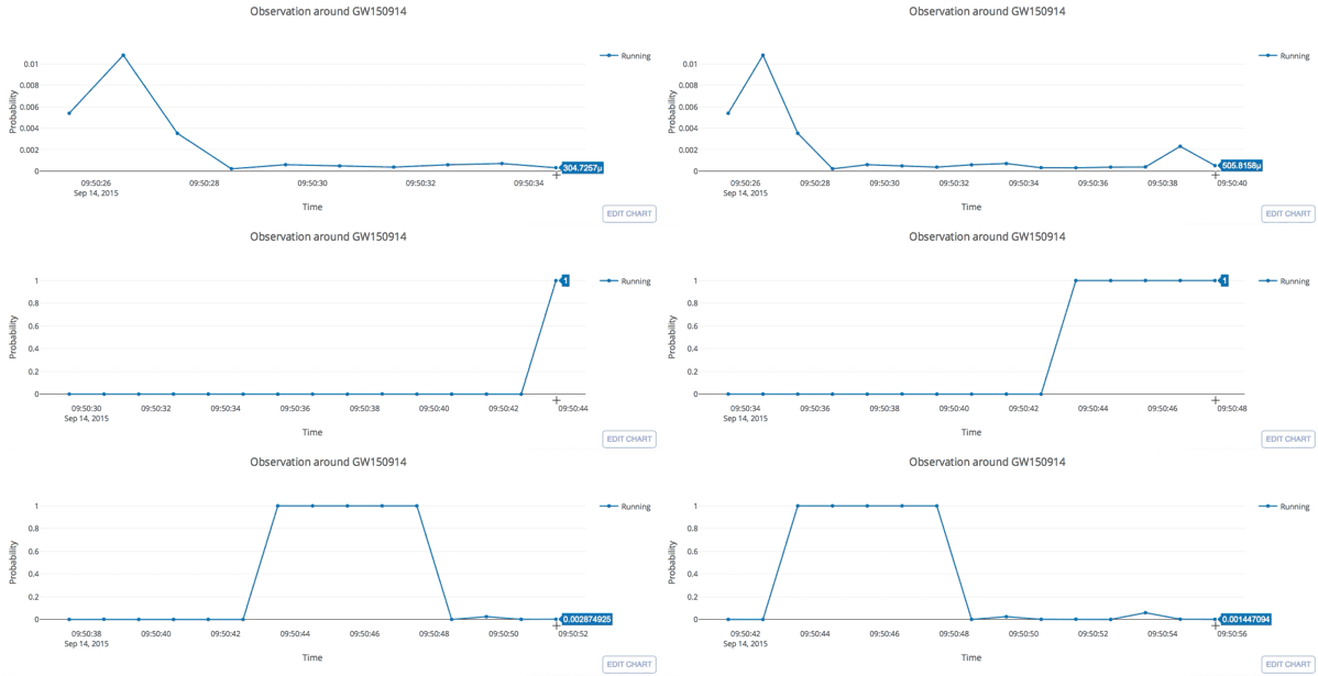
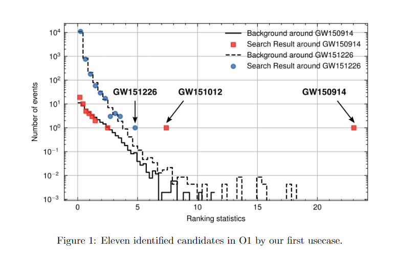
Real-time GW searches for GW150914
H.W., et al. PRD (2020)
Expanding the dimension of the output
CL.M., W.W., H.W., et al. PRD (2023)
Beyond Speed: Generalization and Discovery in GW Detection
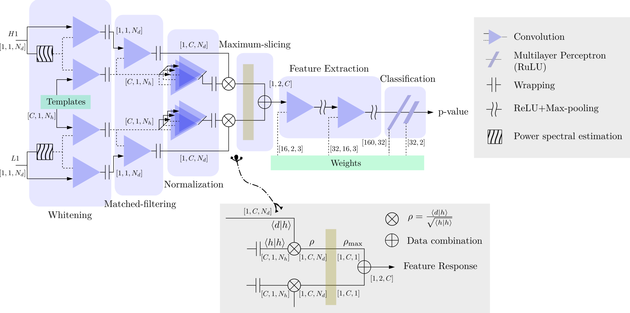
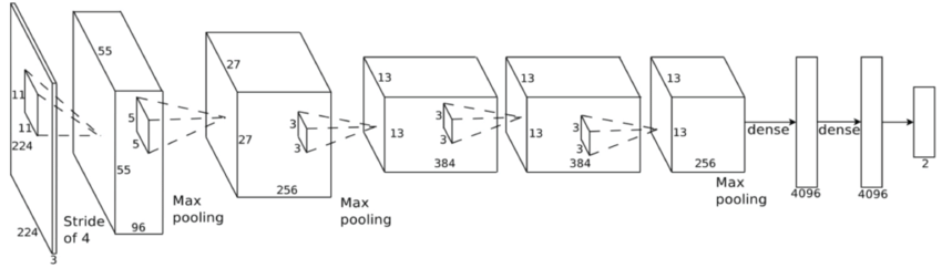
Feature extraction
Convolutional Neural Network (ConvNet or CNN)
Classification
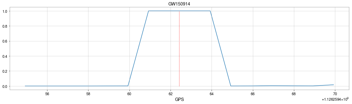
GW150914
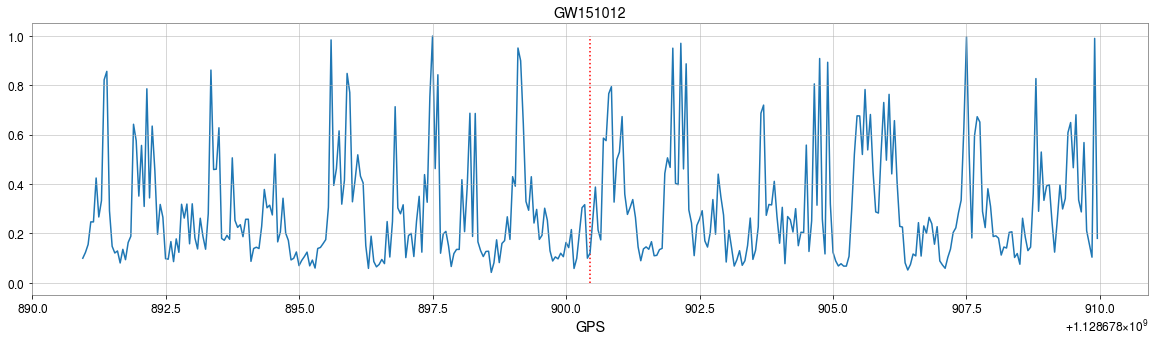
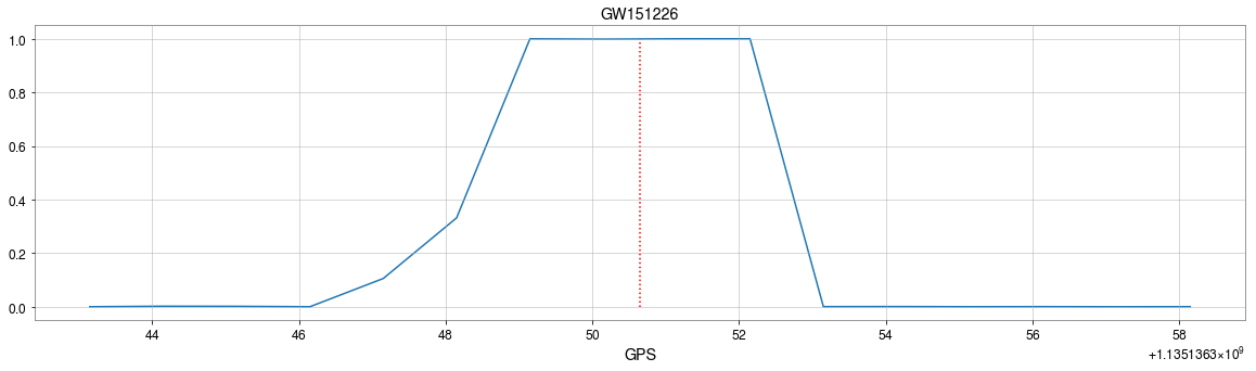
GW151226
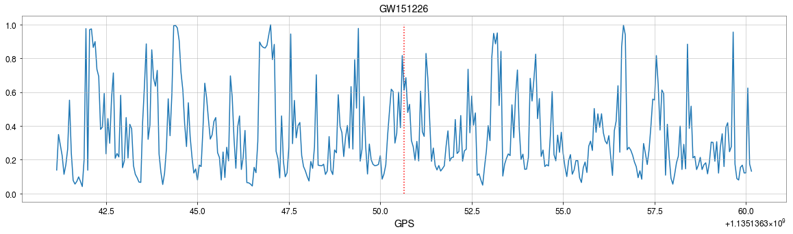
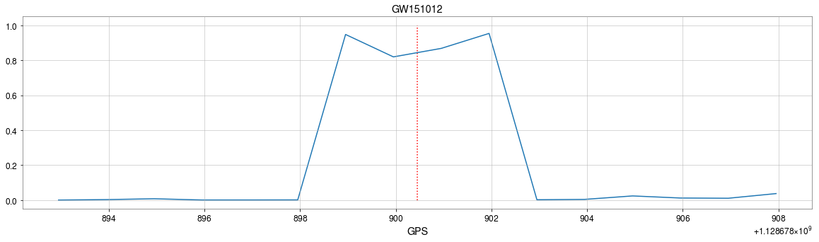
GW151012
>> Is it matched-filtering ?
>> Wait, It can be matched-filtering!
Beyond Speed: Generalization and Discovery in GW Detection
He Wang, et al. PRD 101, 10 (2020): 104003
GW150914
GW151226
GW151012
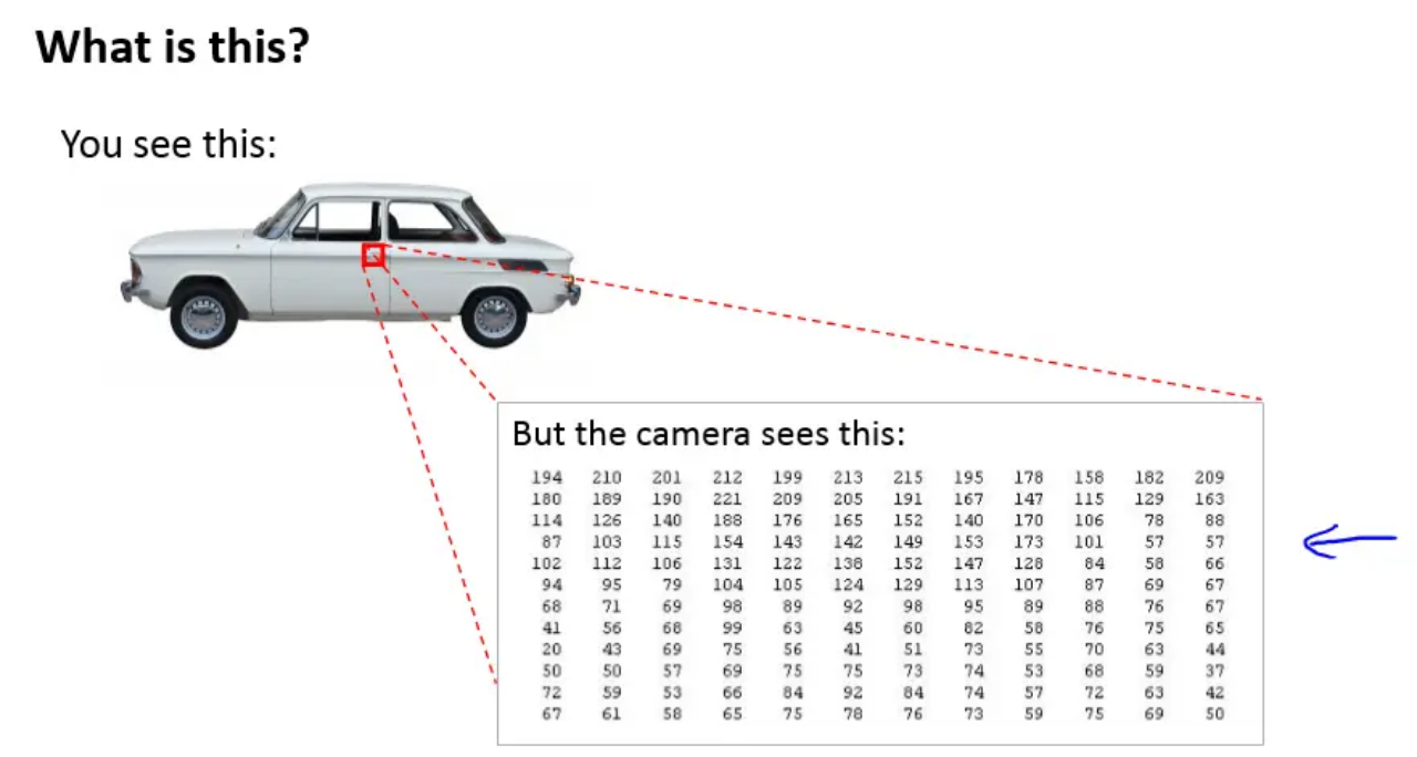
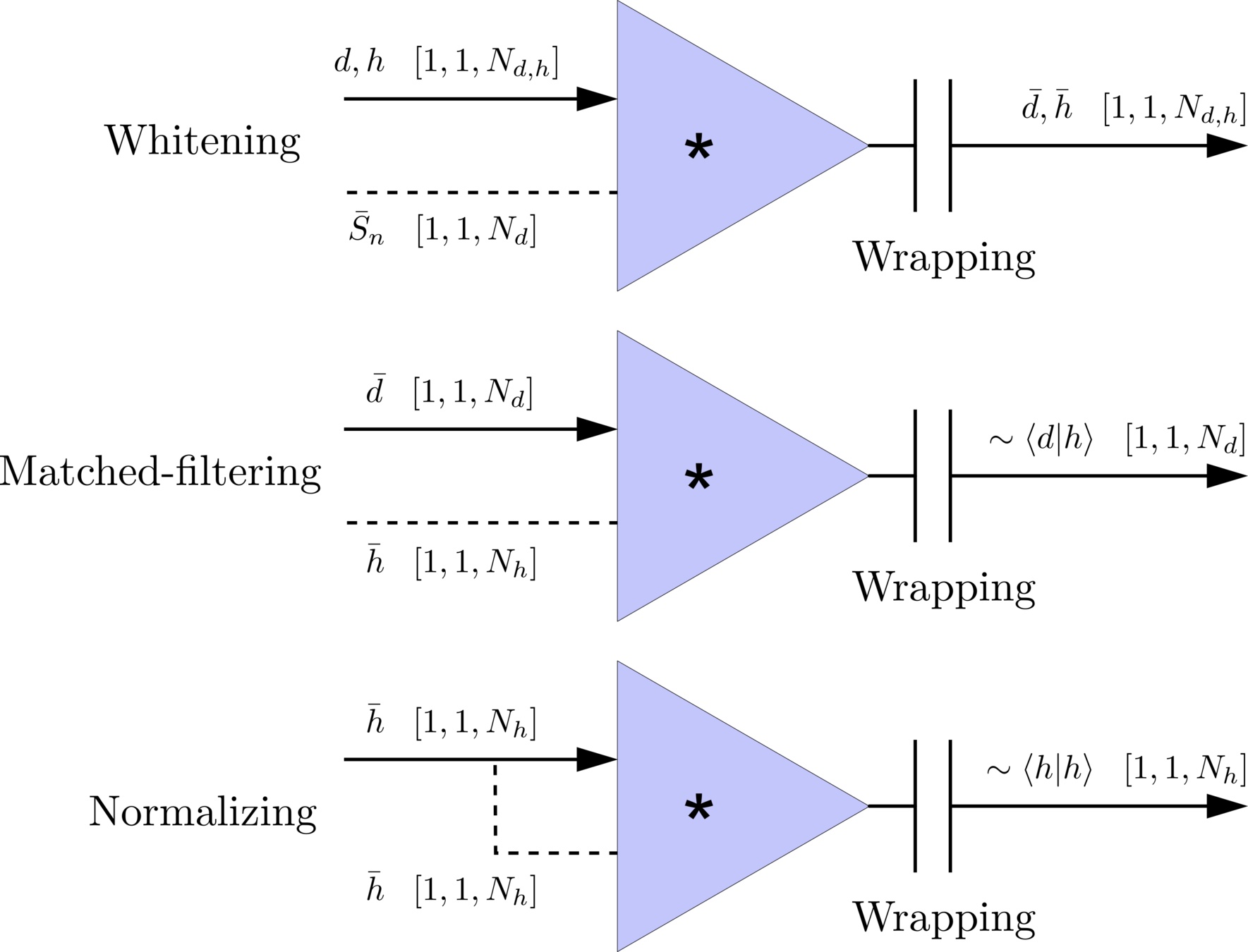
MFCNN MFCNN MFCNNMatched-filtering (cross-correlation with the templates) can be regarded as a convolutional layer with a set of predefined kernels.
Real-time GW searches for GW150914
Beyond Speed: Generalization and Discovery in GW Detection
He Wang, et al. PRD 101, 10 (2020): 104003
Frequency domain
Time domain
(normalizing)
(matched-filtering)
\(S_n(|f|)\) is the one-sided average PSD of \(d(t)\)
(whitening)
where
Deep Learning Framework
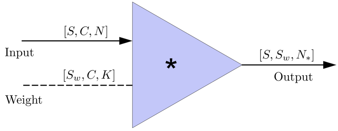
FYI: \(N_\ast = \lfloor(N-K+2P)/S\rfloor+1\)
(A schematic illustration for a unit of convolution layer)
Beyond Speed: Generalization and Discovery in GW Detection
He Wang, et al. PRD 101, 10 (2020): 104003
Frequency domain
Time domain
(normalizing)
(matched-filtering)
\(S_n(|f|)\) is the one-sided average PSD of \(d(t)\)
(whitening)
where
Deep Learning Framework
Beyond Speed: Generalization and Discovery in GW Detection
He Wang, et al. PRD 101, 10 (2020): 104003
import mxnet as mx
from mxnet import nd, gluon
from loguru import logger

def MFCNN(fs, T, C, ctx, template_block, margin, learning_rate=0.003):
    logger.success('Loading MFCNN network!')
    net = gluon.nn.Sequential()
    with net.name_scope():
        net.add(MatchedFilteringLayer(mod=fs*T, fs=fs,
                                      template_H1=template_block[:,:1],
                                      template_L1=template_block[:,-1:]))
        net.add(CutHybridLayer(margin = margin))
        net.add(Conv2D(channels=16, kernel_size=(1, 3), activation='relu'))
        net.add(MaxPool2D(pool_size=(1, 4), strides=2))
        net.add(Conv2D(channels=32, kernel_size=(1, 3), activation='relu'))
        net.add(MaxPool2D(pool_size=(1, 4), strides=2))
        net.add(Flatten())
        net.add(Dense(32))
        net.add(Activation('relu'))
        net.add(Dense(2))
	# Initialize parameters of all layers
    net.initialize(mx.init.Xavier(magnitude=2.24), ctx=ctx, force_reinit=True)
    return net
The available codes (2019): https://gist.github.com/iphysresearch/a00009c1eede565090dbd29b18ae982c
1 sec duration
35 templates used
["This", "is", "a", "sample"]
He Wang et al 2024 Mach. Learn.: Sci. Technol. 5 015046
Strain
Whiten
Normalized
∼\(10^{−19}\)
∼\(10^{2}\)
∼\(10^{0}\)
32 s
32 s
merger
\(t_c\) (around GW150914)
(Cal network SNR)
Band-pass: [20, 2048] Hz
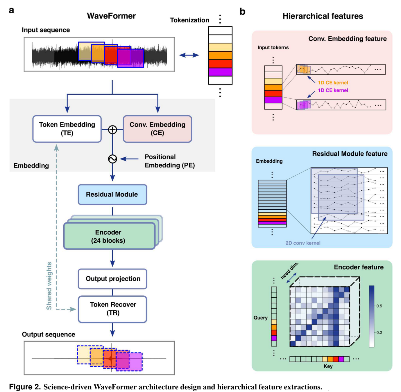
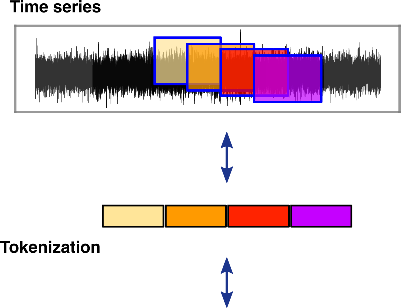
Patching (tokenized) with size 0.125 s and overlap 50%
[1, 128, 256]
(Standard normalization)
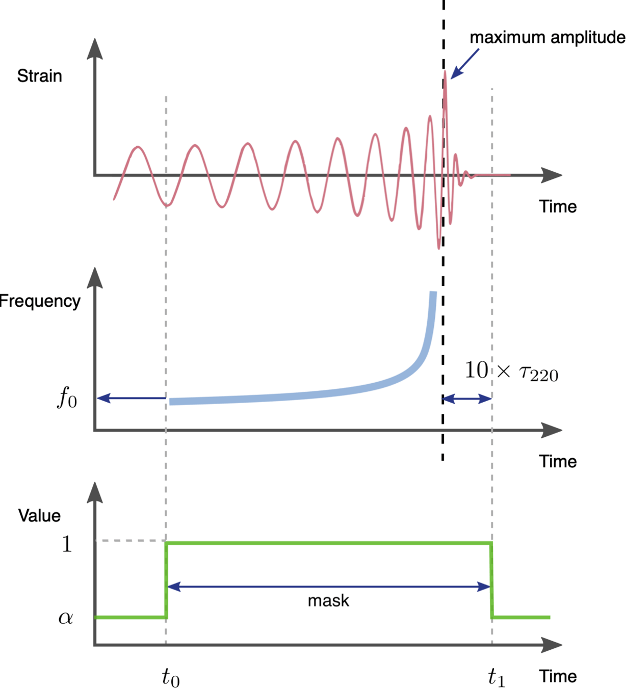
dynamic masking
[1, 16512]
[1, 128, 256]
(PSD\(_i\) from noise)
Band-pass: [20, 2048] Hz
WaveFormer
MSE-Loss\(_i\)
\(std\)
[1, 128, 256]
Noise\(_i\):
Signal\(_i\):
Input\(_i\):
Label\(_i\):
Output\(_i\):
8.0625 s
8.0625 s
Given �=ℎ+�d=h+n, we can normalize �d as follows:
He Wang et al 2024 Mach. Learn.: Sci. Technol. 5 015046
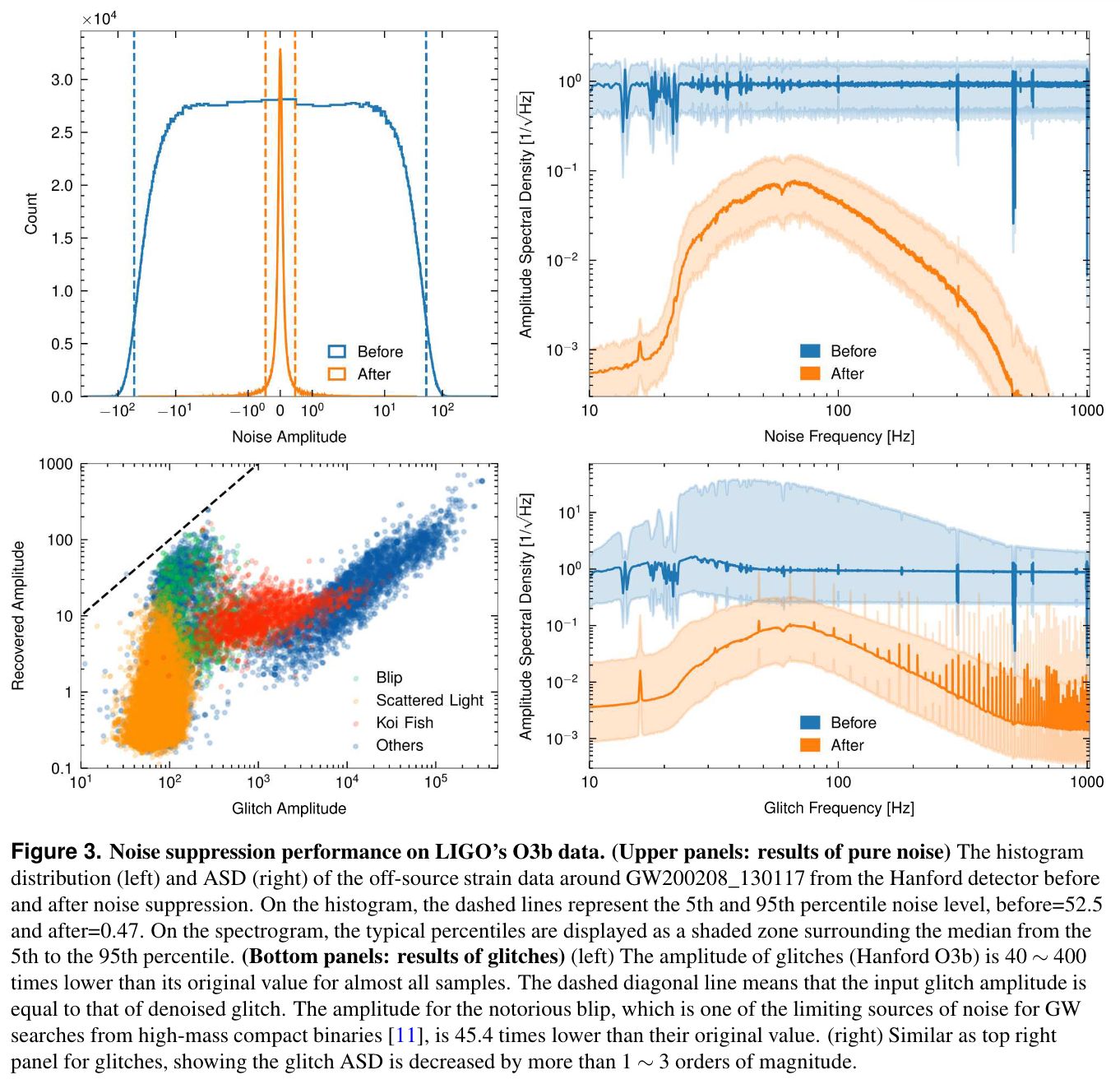
(Bottom panels: results of glitches)
(Upper panels: results of pure noise)
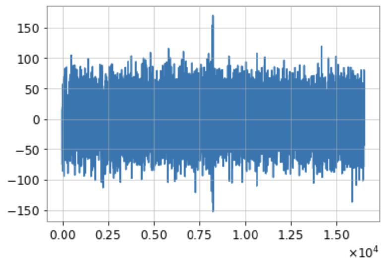
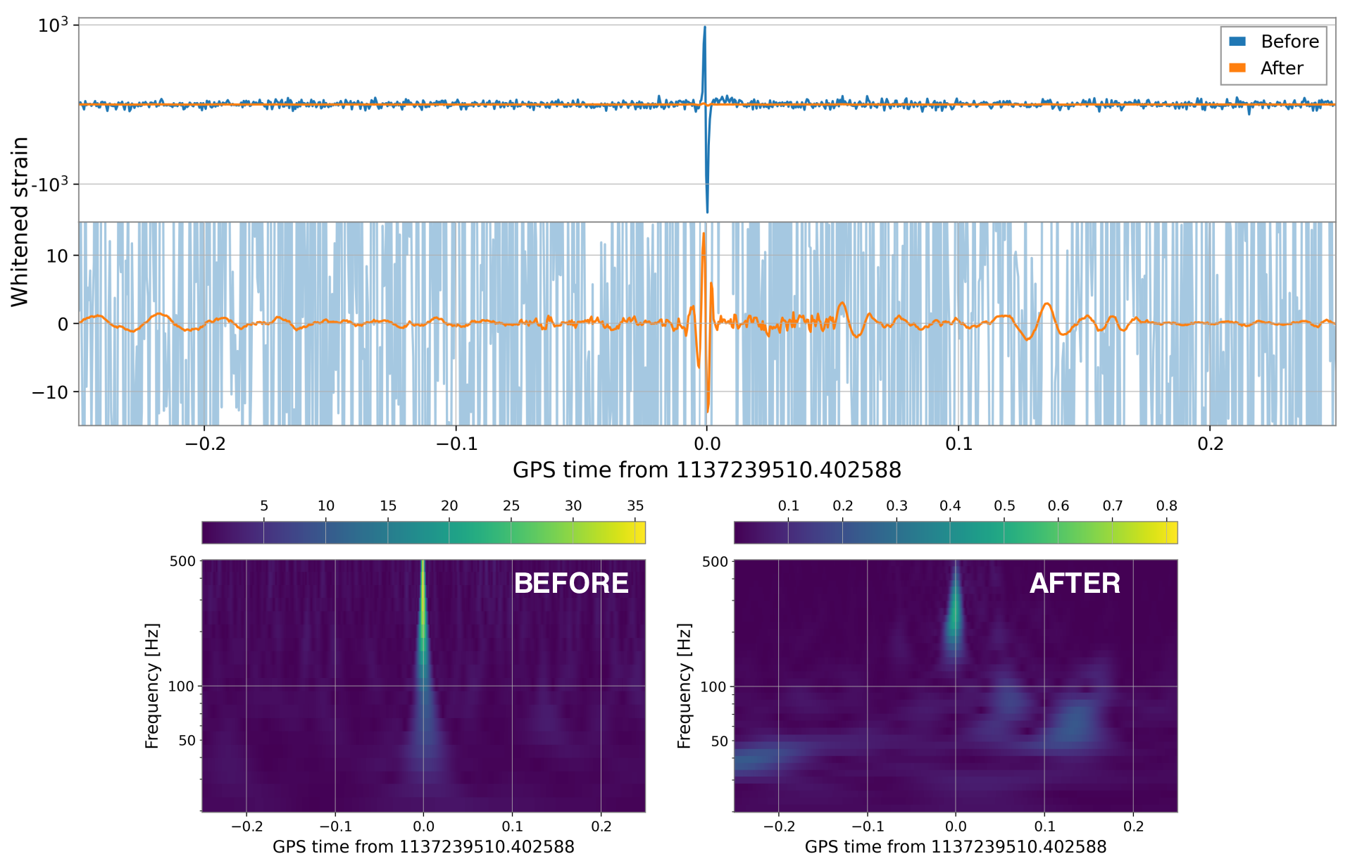
Time-series and spectrogram example of blip.
He Wang et al 2024 Mach. Learn.: Sci. Technol. 5 015046
(Upper panels: Signal amplitude recovery performance
(Bottom panels: Signal phase recovery performance)
Bacon P. et al. arXiv: 2205.13513
He Wang et al 2024 Mach. Learn.: Sci. Technol. 5 015046
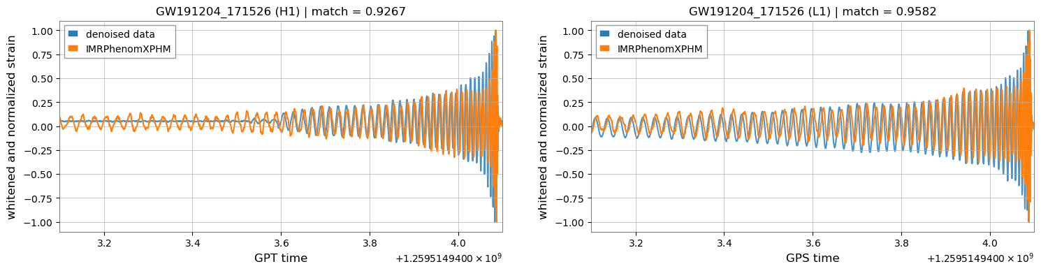
GW191204_171526
He Wang et al 2024 Mach. Learn.: Sci. Technol. 5 015046
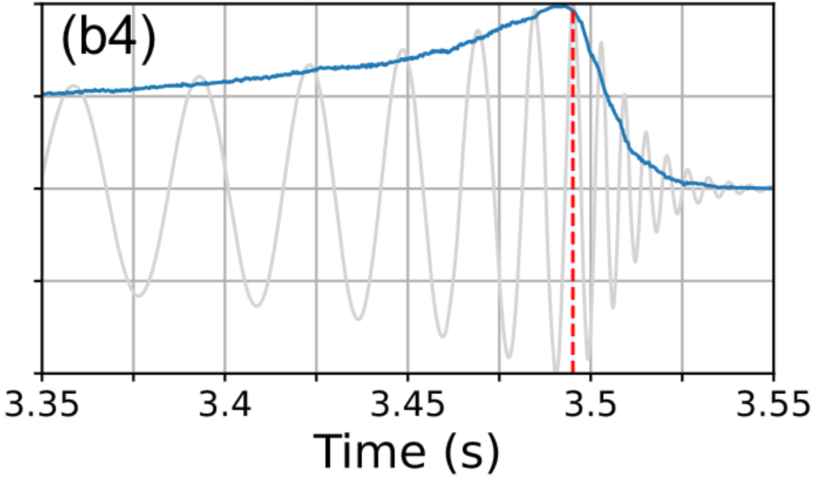
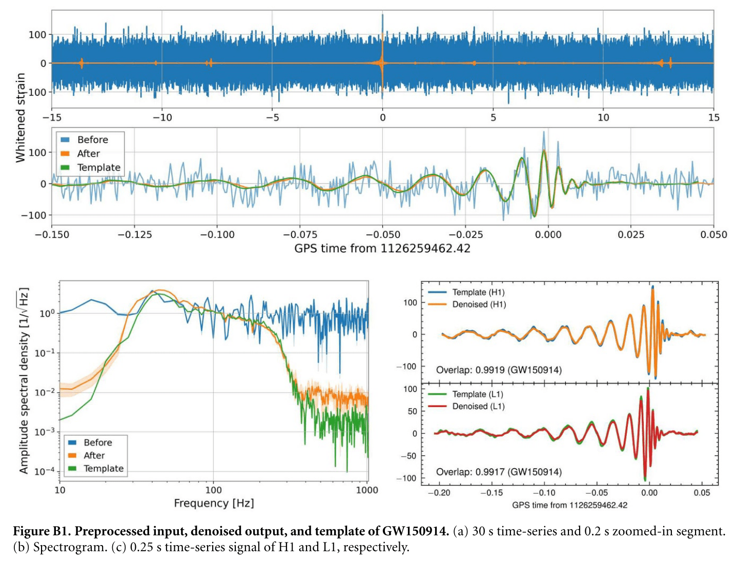
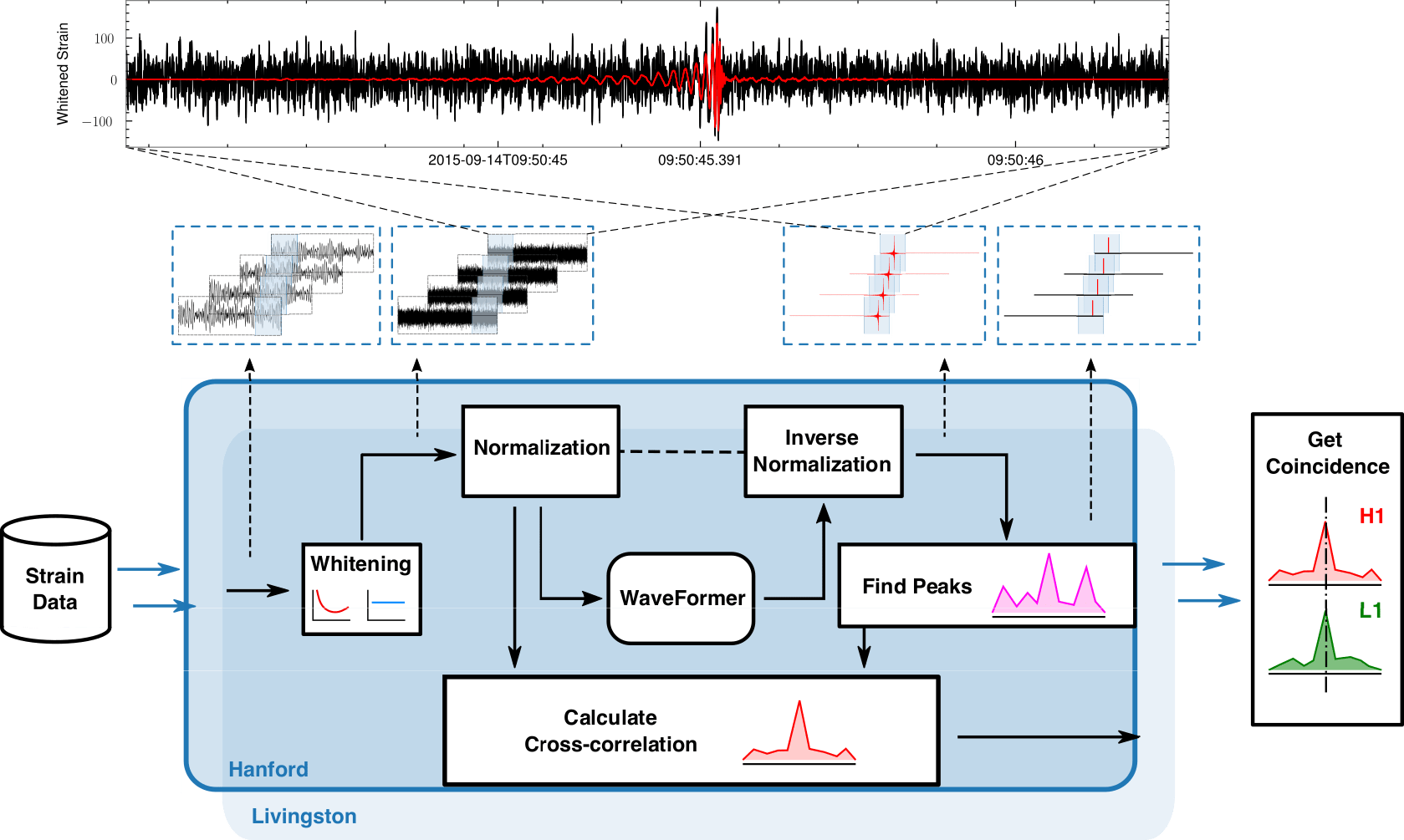
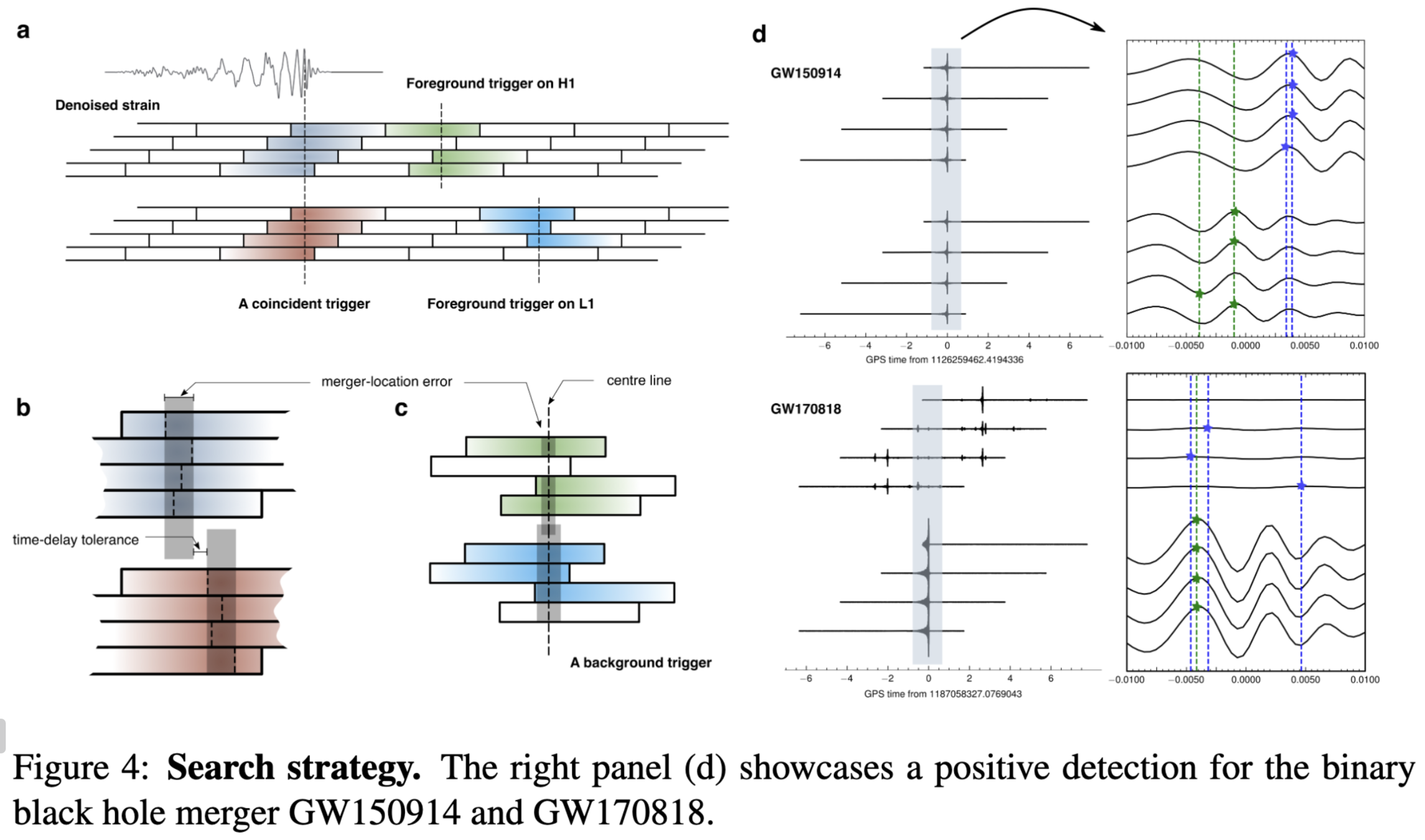
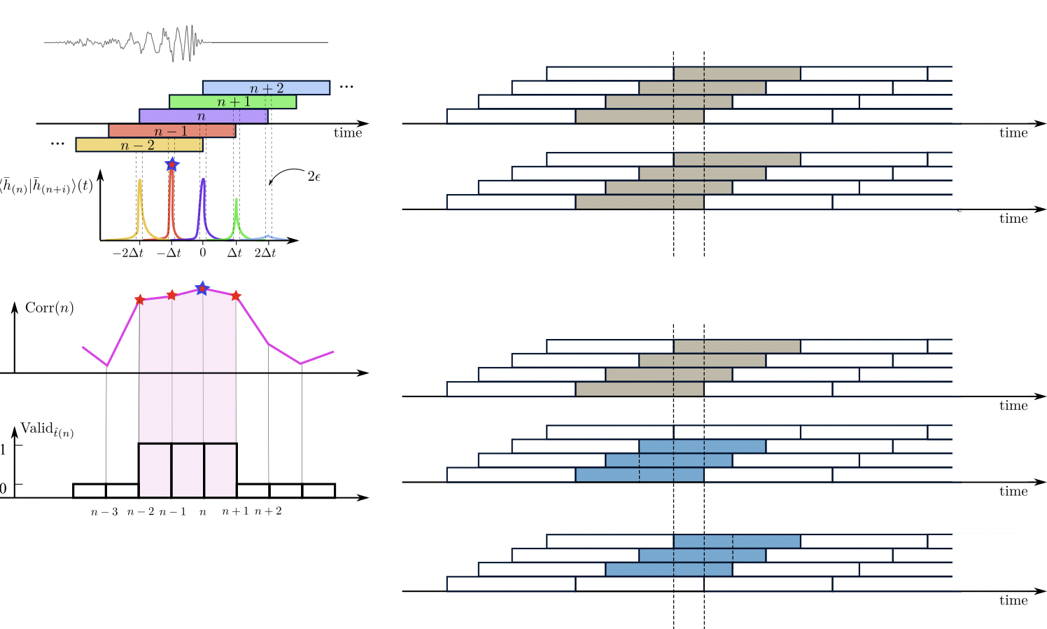
Firstly, we obtain the denoised output by utilizing Waveformer. Then, triggers are defined and identified by three steps including,
Find Peaks. Locate triggers on a single detector by finding its maximum all local-maximum (0.2s away from neighboring maximum/local-maximum).
An search algorithm for GW require that: [cite: 2010.07244]
the same signal is seen in the detectors; (the same signal is seen by time-shifting in single detector)
the same waveform must be present both detectors;
and the signal’s time of arrival must be consistent with the GW travel time between the observatories.
He Wang et al 2024 Mach. Learn.: Sci. Technol. 5 015046
Firstly, we obtain the denoised output by utilizing Waveformer.
Then, triggers are defined and identified by three steps including:
Find Peaks. Locate triggers on a single detector by finding its maximum all local-maximum (0.2s away from neighboring maximum/local-maximum).
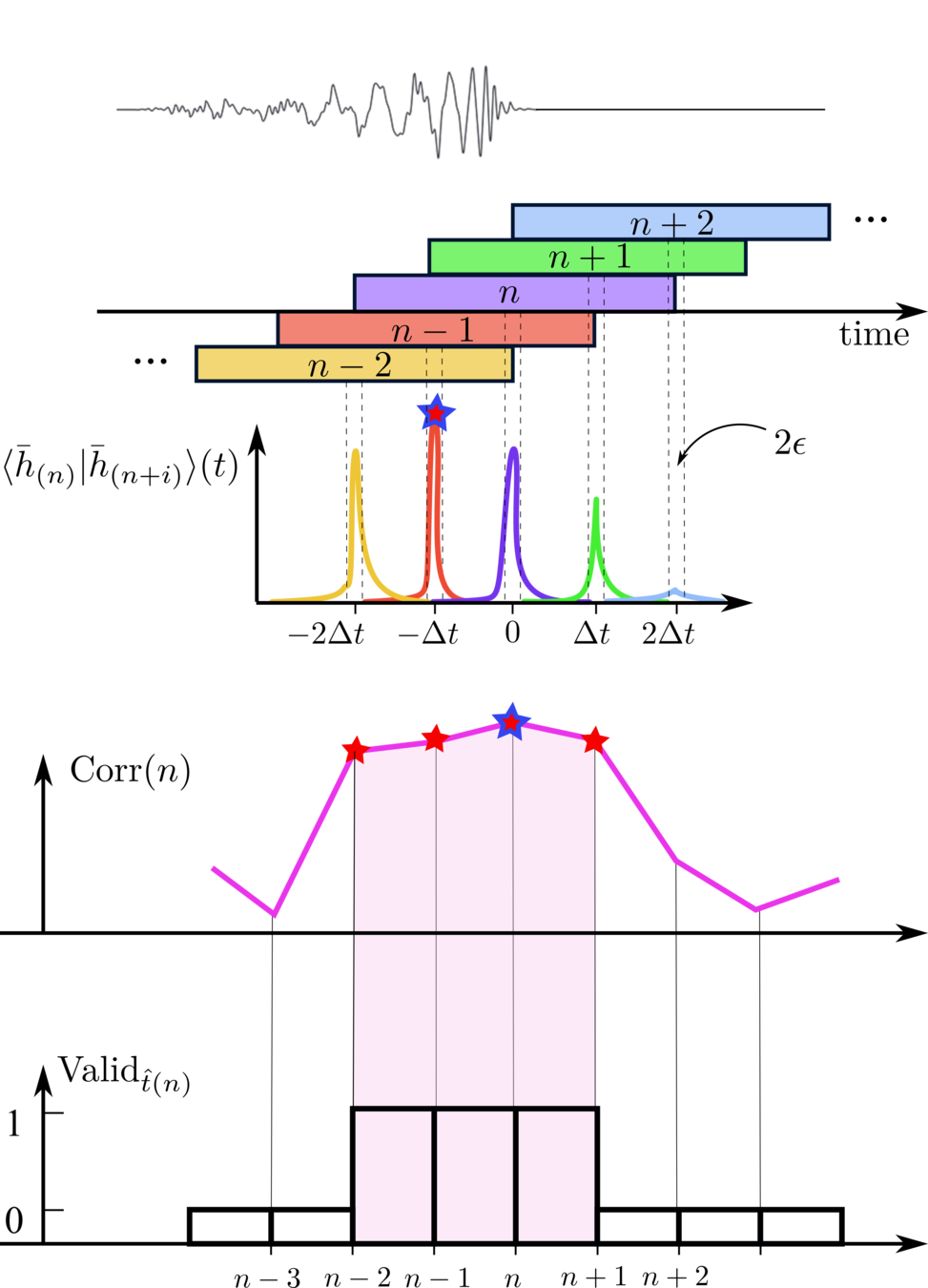
By constraining triggers that exist on both two detectors, we get VALID triggers. (consist 3~4 segments)
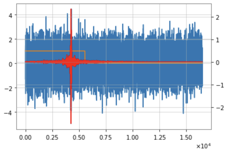
Calculate the cross-correlation of the to-be-evaluated trigger across channels or within a single channel, between its noisy and corresponding denoised segments, as well as between denoised segments themselves.
noisy input segments
denoised output segments
\(\bar{H}\)
\(\bar{L}\)
\({H}\)
\({L}\)
AI
He Wang et al 2024 Mach. Learn.: Sci. Technol. 5 015046
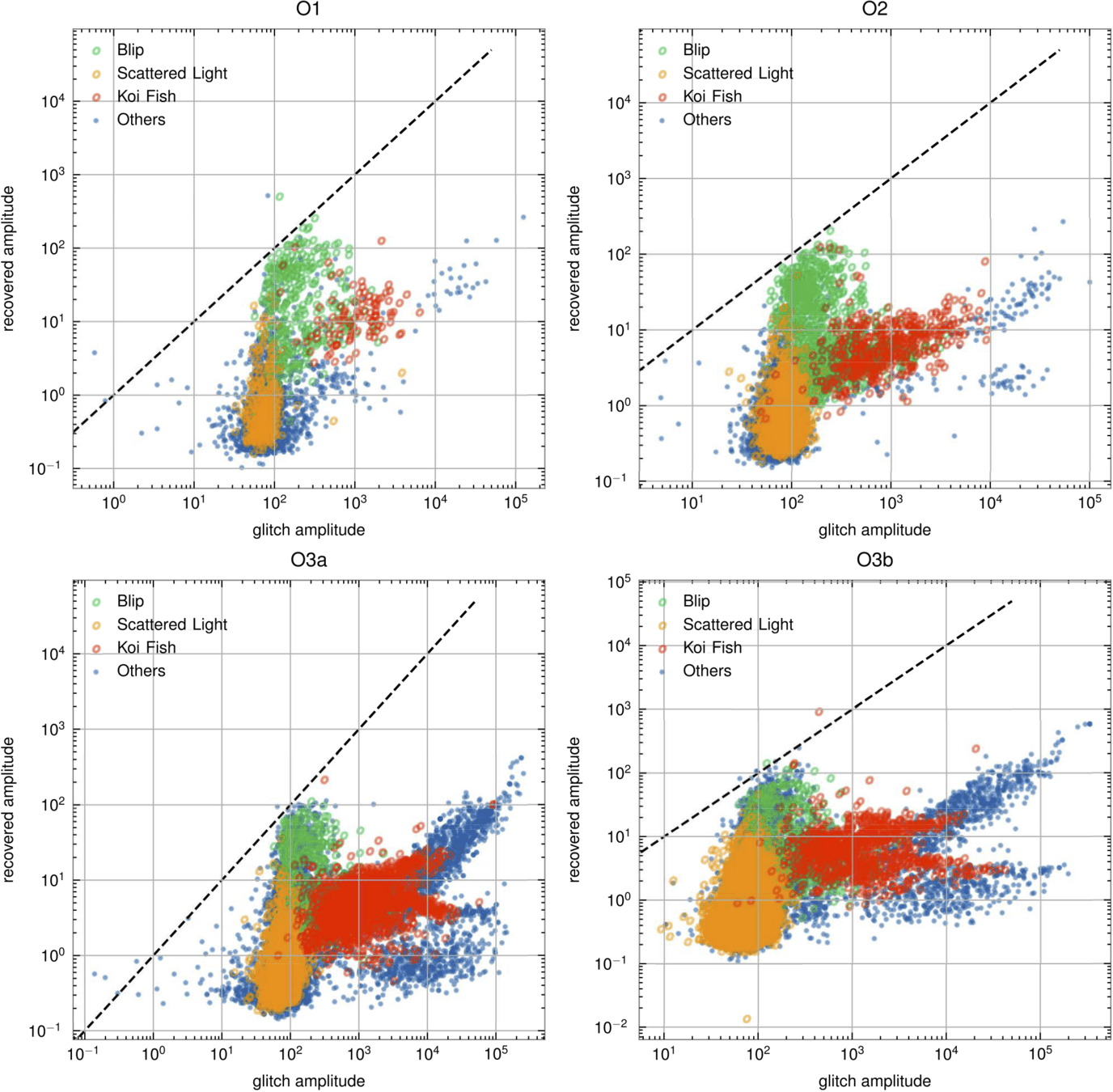
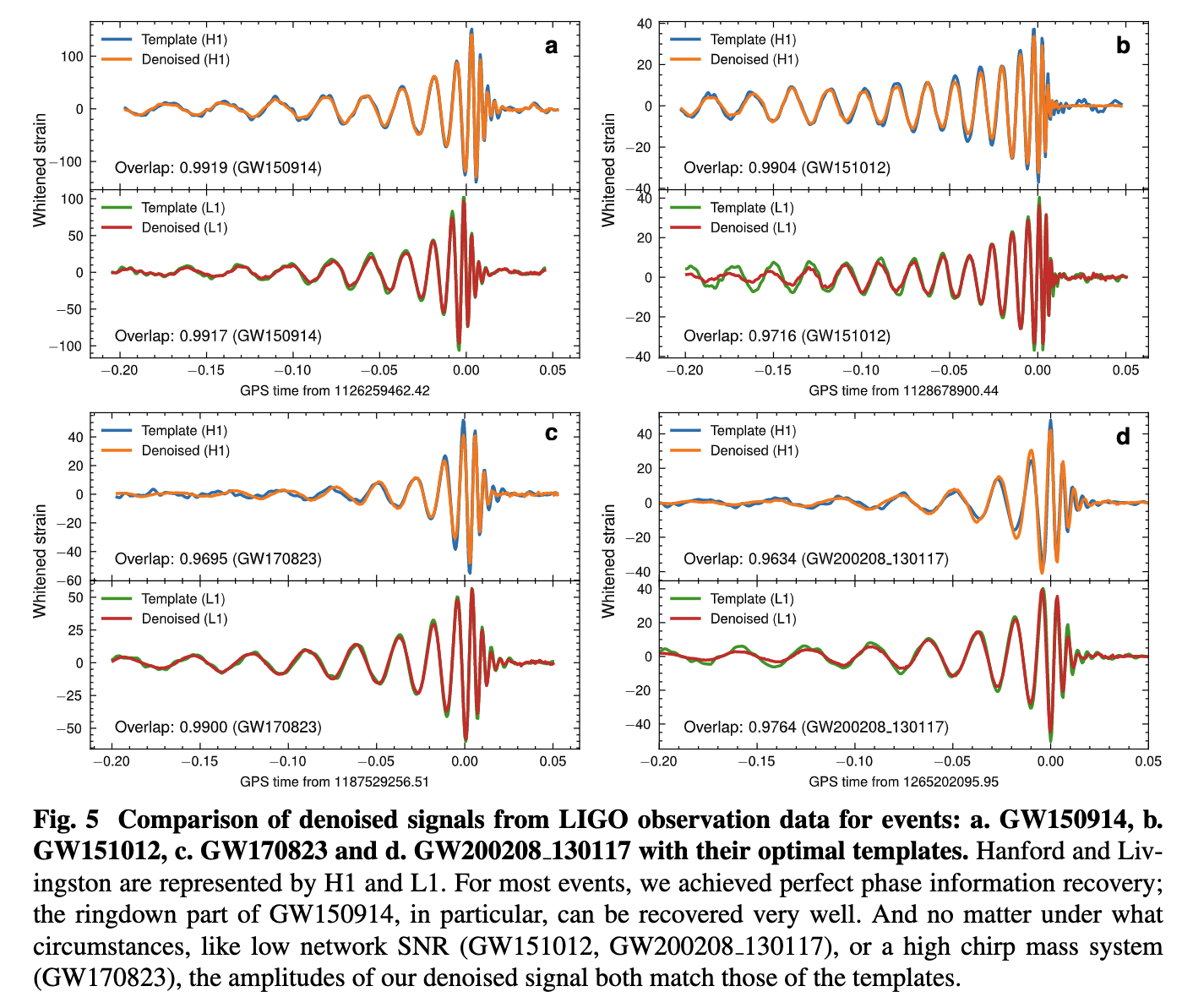
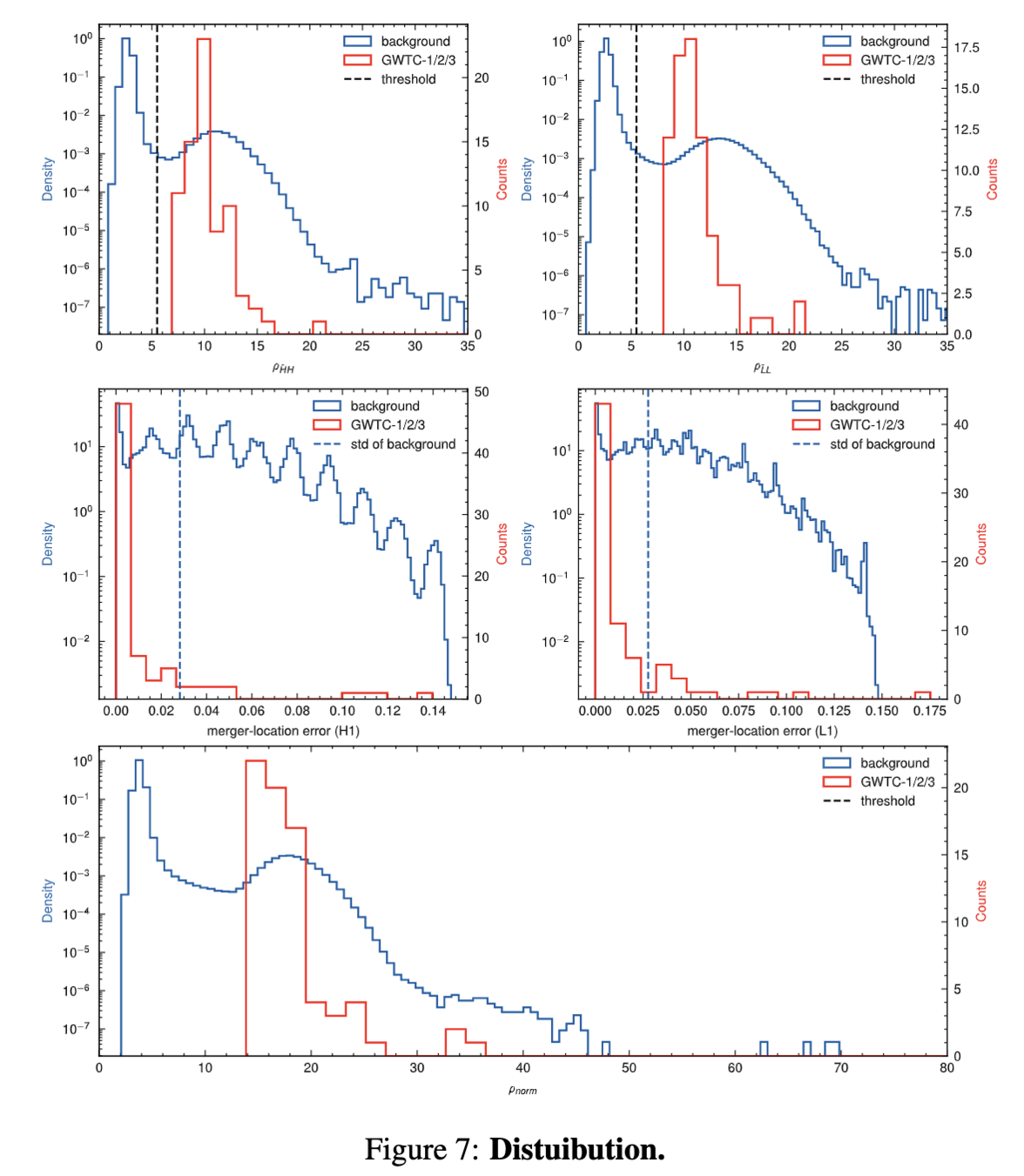
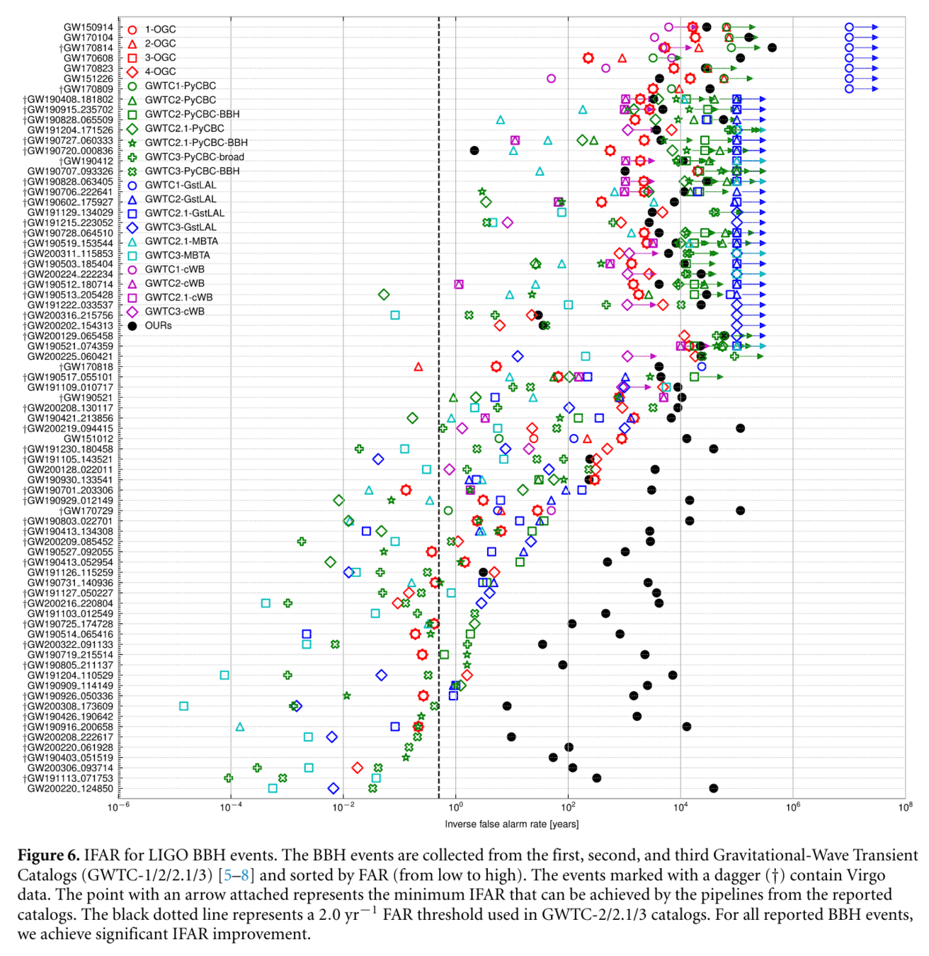
Assessed denoising workflow performance by comparing with GWTC-1, GWTC-2, GWTC2.1, and GWTC-3 catalogs and associated data releases.
Noted significant divergence in IFAR distribution between our results and those from GWTC and OGC catalogs.
Achieved significant IFAR improvement across all 75 reported BBH events, indicating effective suppression of loud terrestrial noise.
Example: For low SNR (\(10.8_{-0.4}^{+0.3}\)) event GW200208_130117, obtained an IFAR of 8916 years, surpassing maximum IFAR of <4000 years in other catalogs.
Variability in IFAR improvement linked to the original data's noise nature, including its non-Gaussian, non-stationary characteristics, and different signal recognition strategies by pipelines.
IFAR performance significantly depends on the reduction of non-Gaussian noise near each event.
Events with substantial IFAR improvement had misleading non-Gaussian noise effectively eliminated.
Events where IFAR underperforms retained non-Gaussian characteristics, possibly due to WaveFormer's inherent systematic errors.
He Wang et al 2024 Mach. Learn.: Sci. Technol. 5 015046
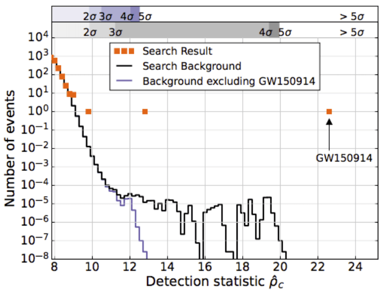
LVK. PRD (2016). arXiv:1602.03839
GW151226
GW151012
He Wang et al 2024 Mach. Learn.: Sci. Technol. 5 015046
PRL 127, 24 (2021) 241103.
PRL 130, 17 (2023) 171403.
Nature Physics 18, 1 (2022) 112–17
He Wang, et al. Big Data Mining and Analytics 5, 1 (2021) 53–63.
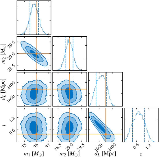
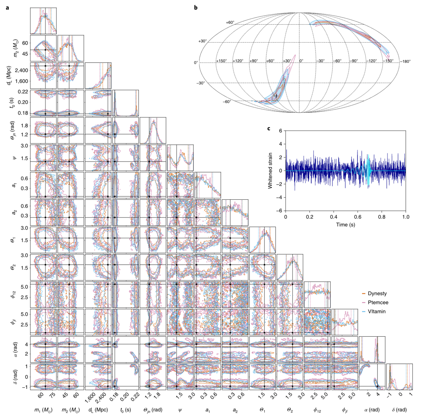
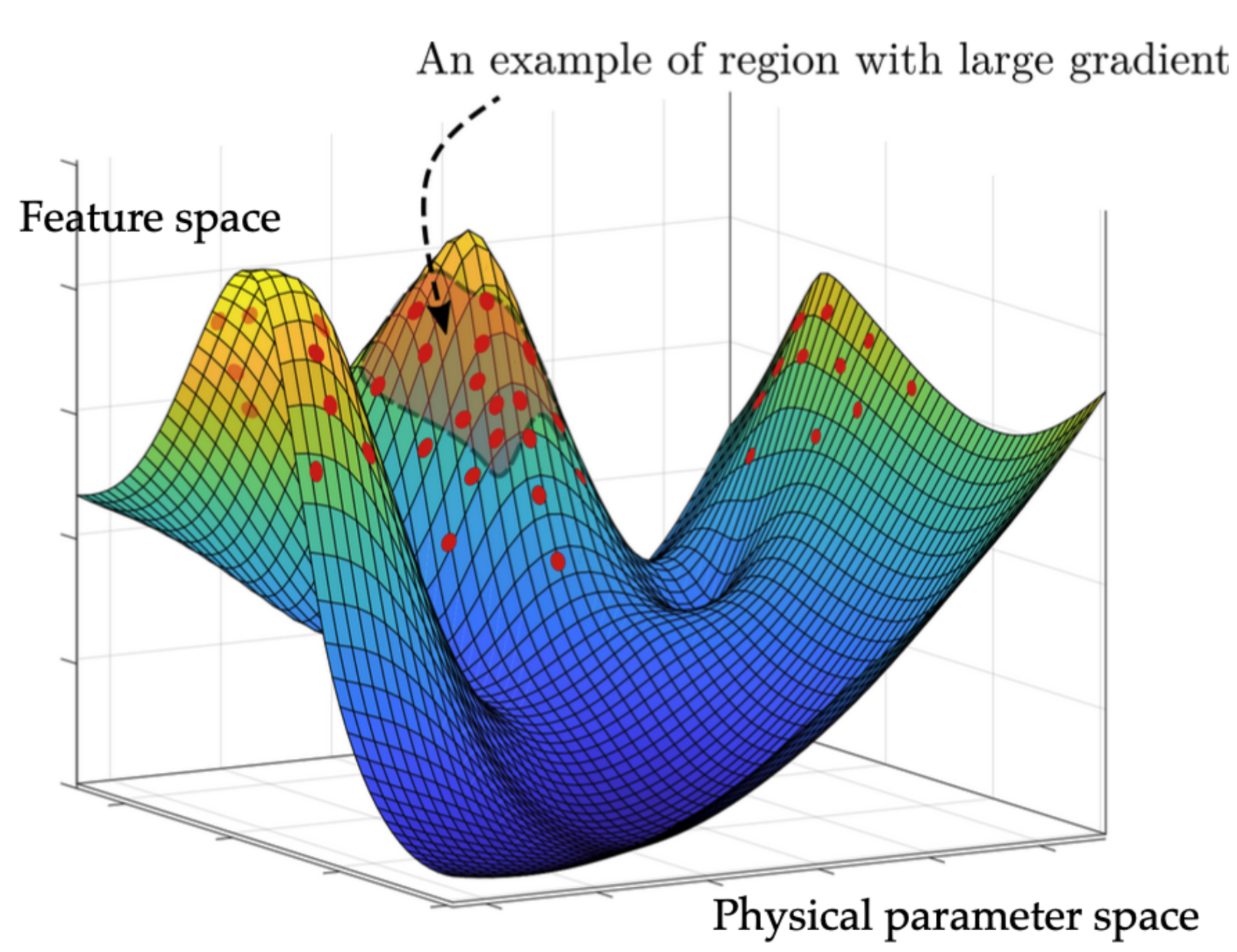
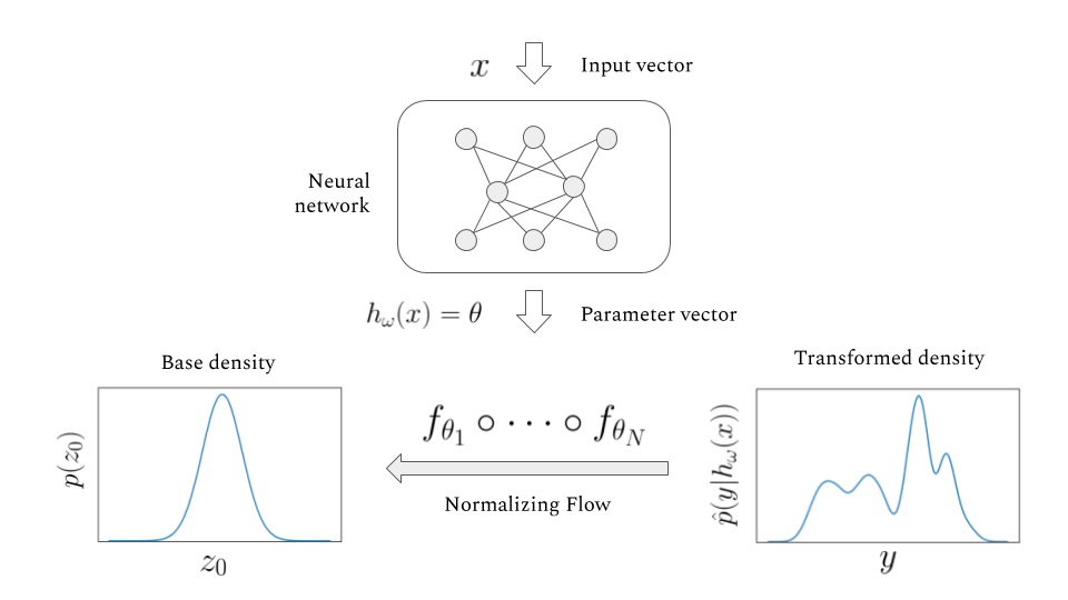
A diagram of prior sampling between feature space and physical parameter space
(Based on 1912.02762)
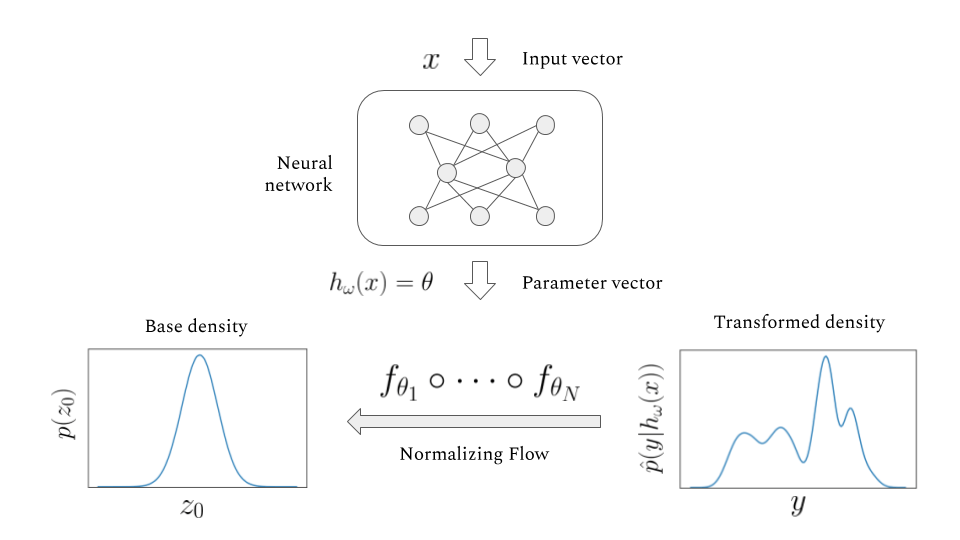
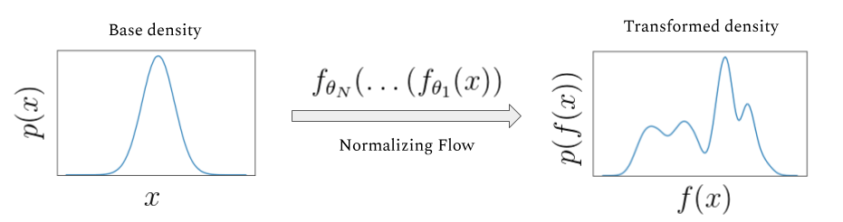
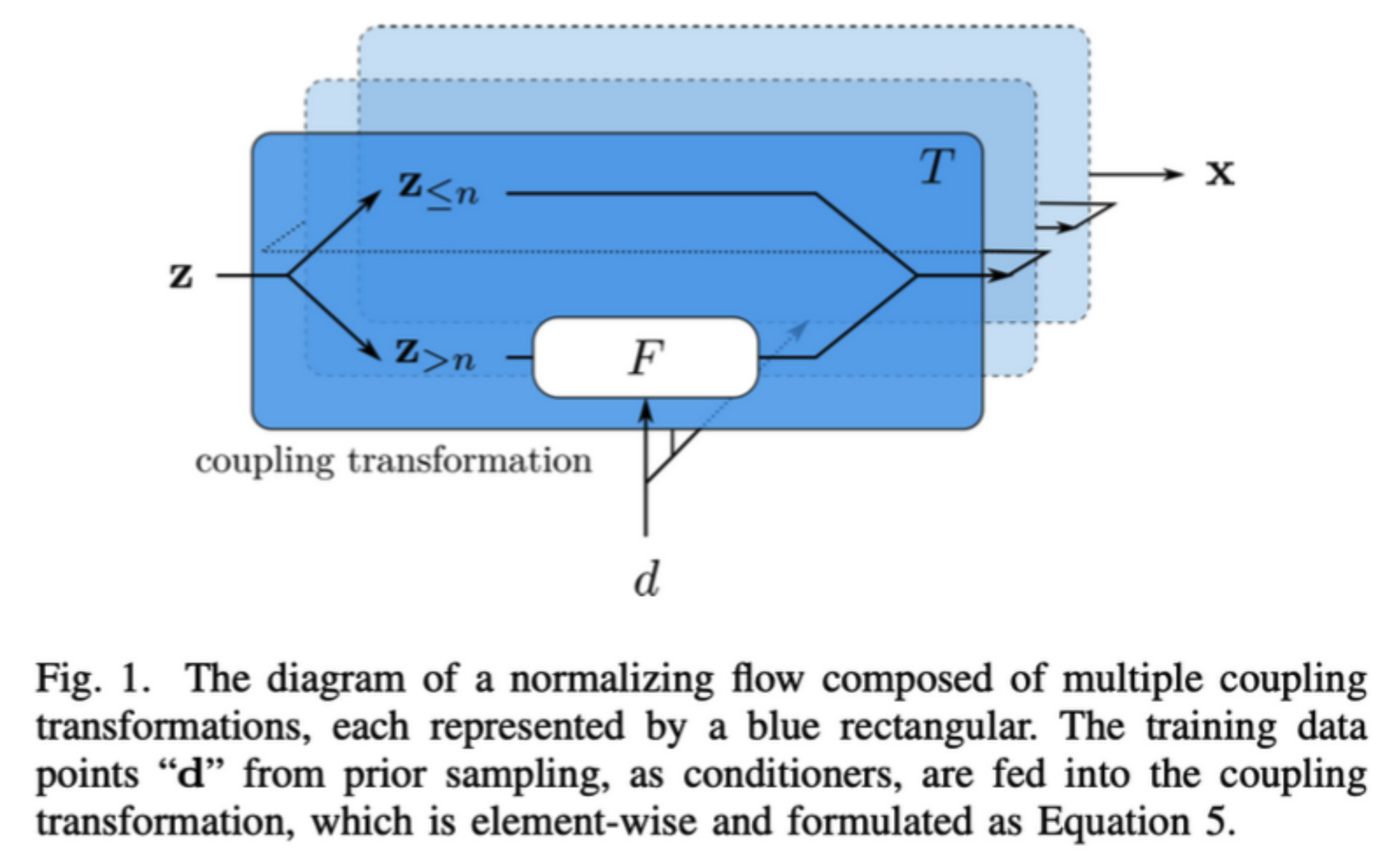
The main idea of flow-based modeling is to express \(\mathbf{y}\in\mathbb{R}^D\) as a transformation \(T\) of a real vector \(\mathbf{z}\in\mathbb{R}^D\) sampled from \(p_{\mathrm{z}}(\mathbf{z})\):
Note: The invertible and differentiable transformation \(T\) and the base distribution \(p_{\mathrm{z}}(\mathbf{z})\) can have parameters \(\{\boldsymbol{\phi}, \boldsymbol{\psi}\}\) of their own, i.e. \( T_{\phi} \) and \(p_{\mathrm{z},\boldsymbol{\psi}}(\mathbf{z})\).
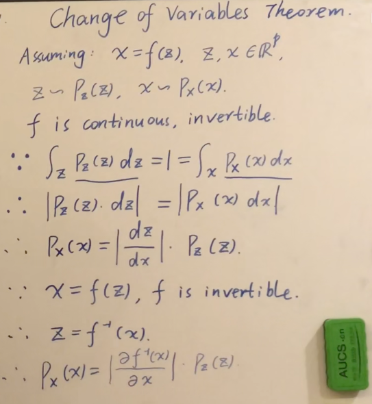
Change of Variables:
Equivalently,
The Jacobia \(J_{T}(\mathbf{u})\) is the \(D \times D\) matrix of all partial derivatives of \(T\) given by:
base density
target density
base density
target density
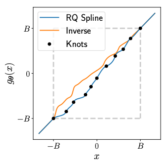
Rational Quadratic Neural Spline Flows
(RQ-NSF)
(Based on 1912.02762)
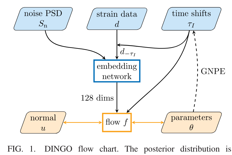
Simulation-Based Inference (SBI)
PRL 127, 24 (2021) 241103.
PRL 130, 17 (2023) 171403.
Real-time gravitational wave science with neural posterior estimation
Sampling with prior knowledge for high-dimensional gravitational wave data analysis
He Wang, et al. Big Data Min. Anal. (2021)
PRD 108, 4 (2023): 044029.
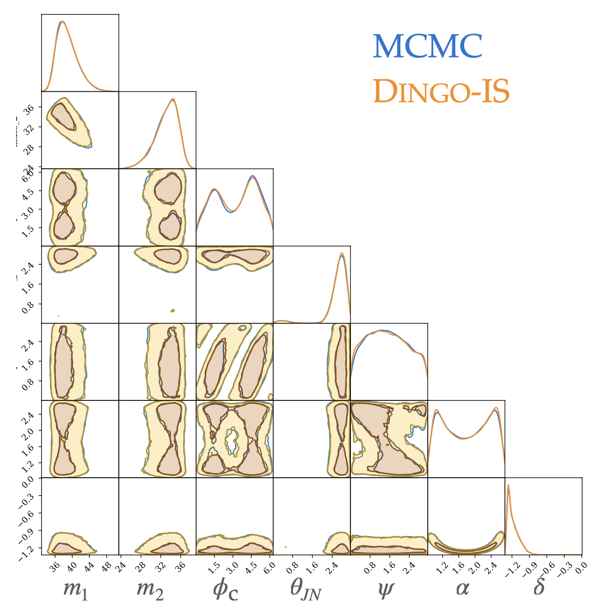
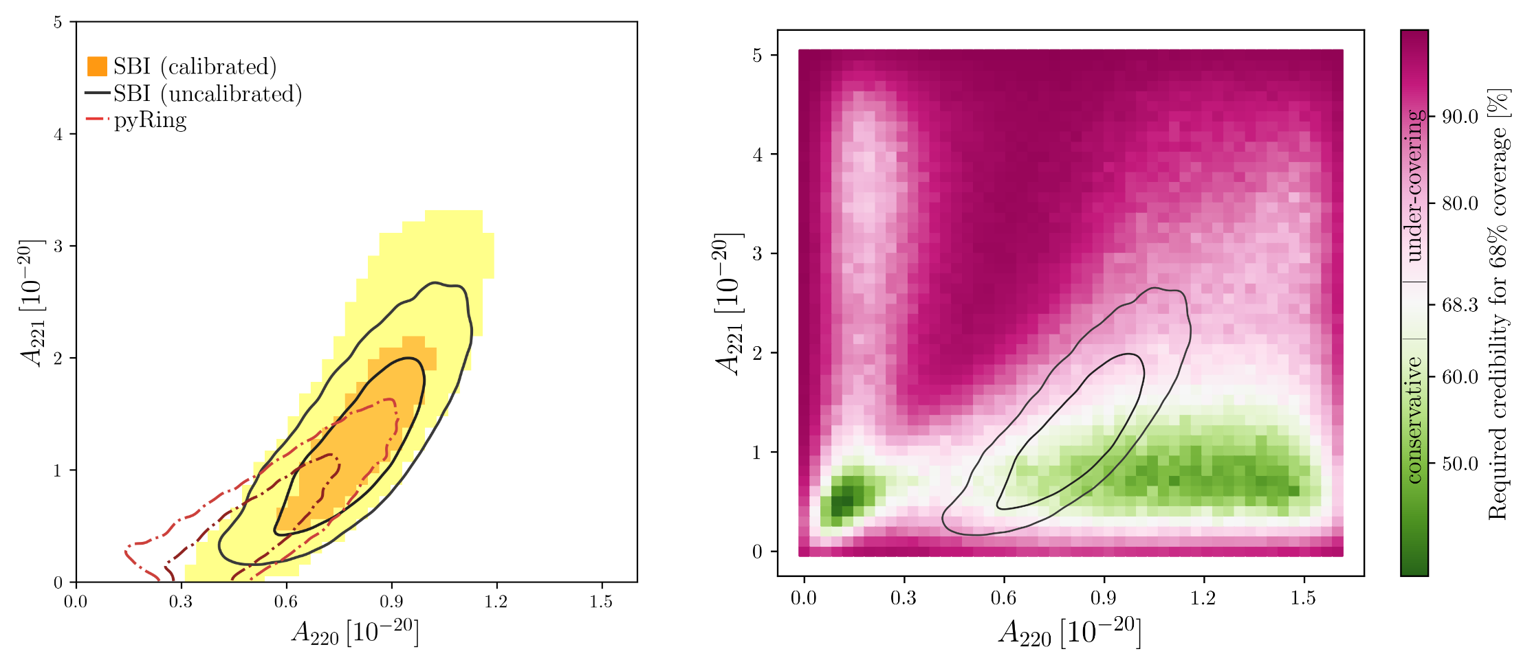
Neural Posterior Estimation with Guaranteed Exact Coverage: The Ringdown of GW150914
arXiv:2310.13405, LIGO-P2300306
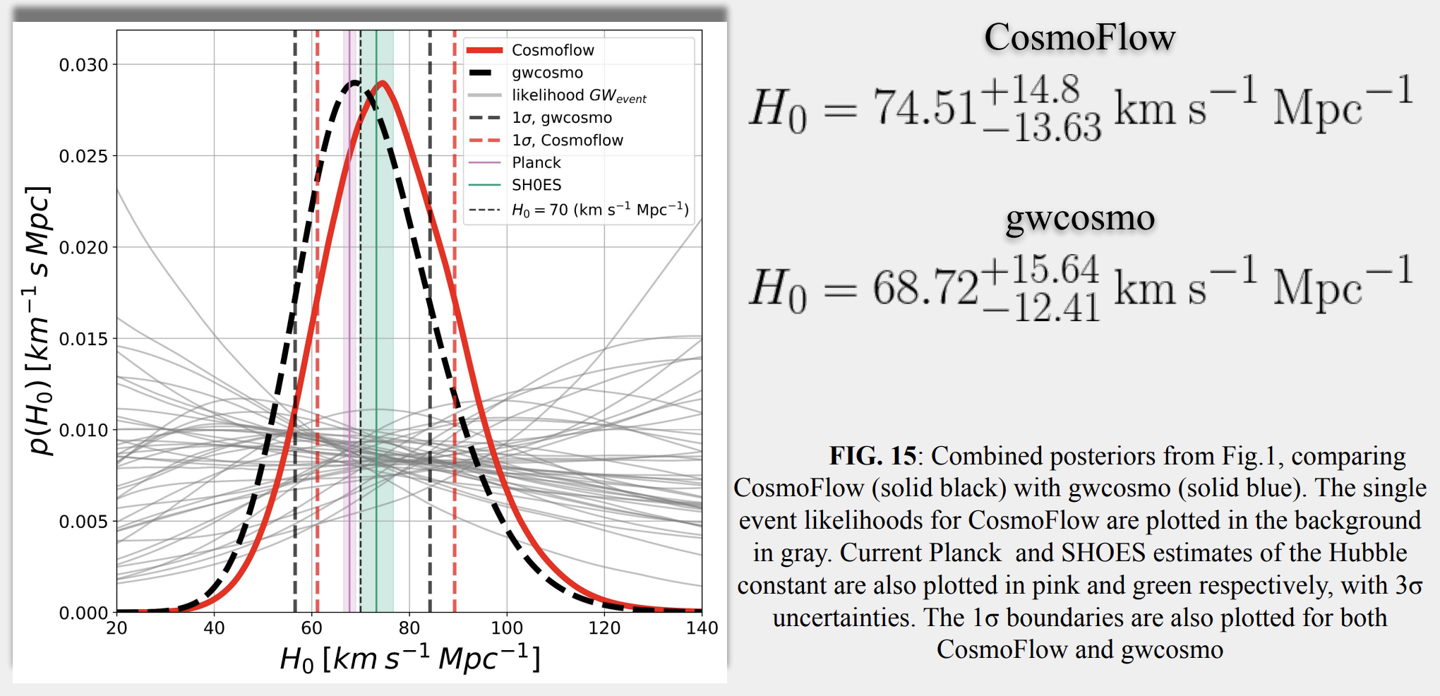
Cosmological Inference using Gravitational Waves and Normalising Flows
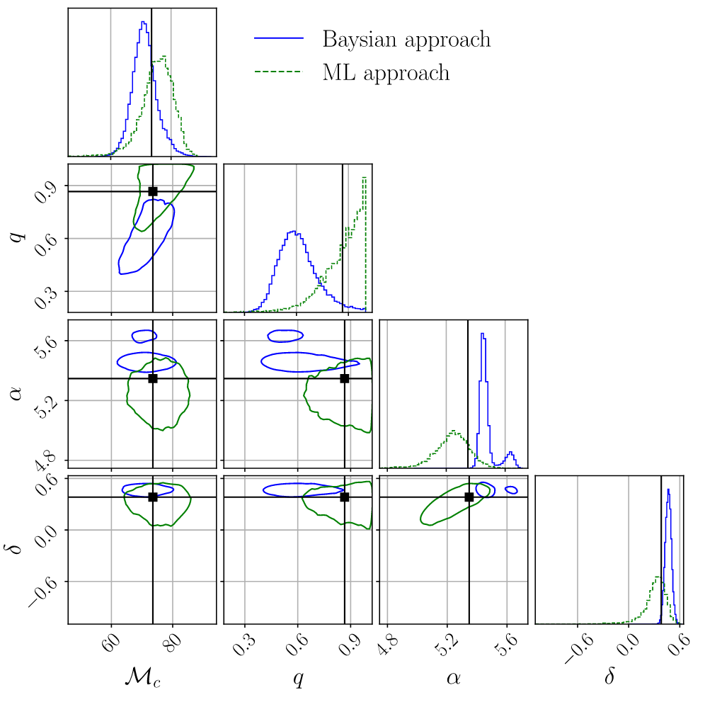
Normalizing Flows as an Avenue to Studying Overlapping Gravitational Wave Signals
arXiv:2310.12209
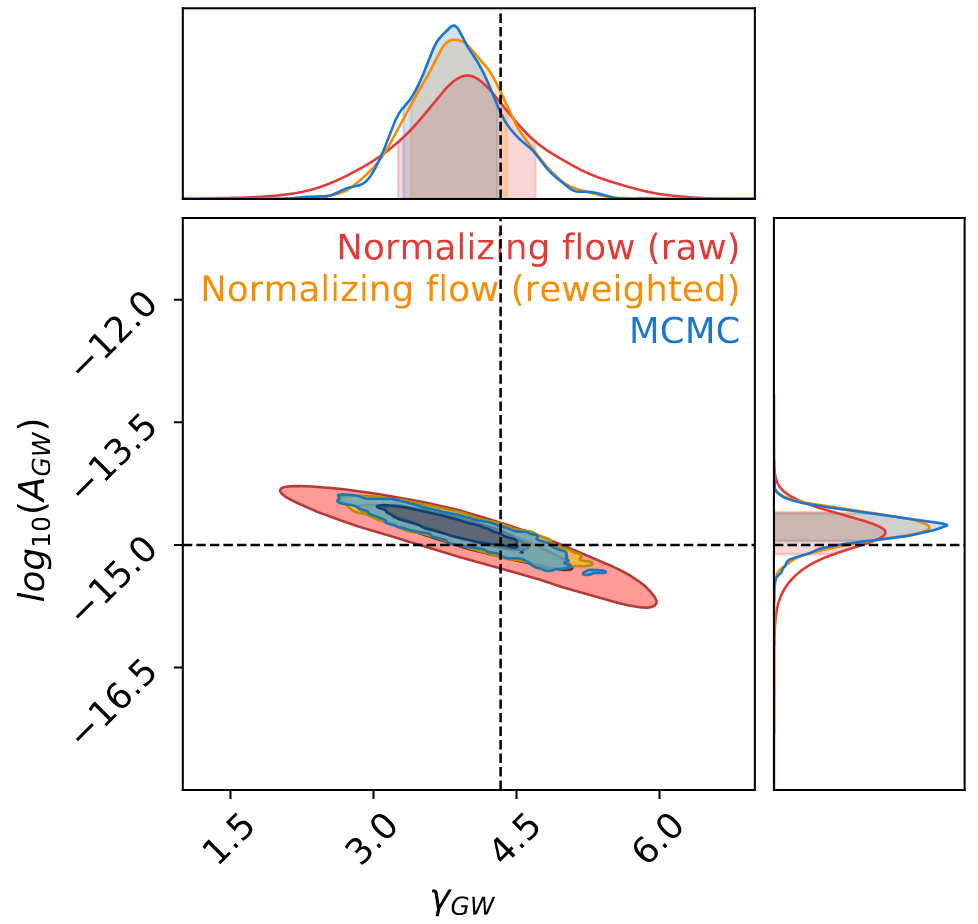
Fast Parameter Inference on Pulsar Timing Arrays with Normalizing Flows
arXiv:2404.14286
Analyses cannot treat sources independently and sequentially work through a list of candidate detections.
The analysis of scientific data from space-based GW detection differs significantly from ground-based detection:
(Sec.8.6 LISA Definition Study Report)
Global vs. Individual Analysis: While global-fit techniques effectively manage the dense overlapping of signals in space-based GW data, individual pipelines are crucial for detecting unique events.
Role of Individual Pipelines: These pipelines act as a pre-processing step, focusing on particular types of sources and diving deeper into the data. They refine the analysis by working on the latest best-fit residuals from the global fit.
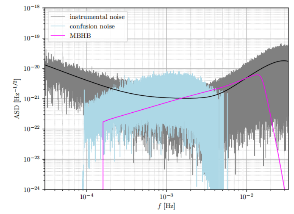
Case Study - MBHB Mergers: Mergers of MBHBs often exhibit high SNR between \(10^2\) to \(10^3\), appearing as distinct peaks in data time series.
Data curation
Model: frequency domain; PhenomD; TDI-A/E response
Input: 1 day length; 15Hz; shape=(2, 3, 2877)
Noise: Gaussian stationary from the noise PSD (for training/test) + GB confusion noise (for test)
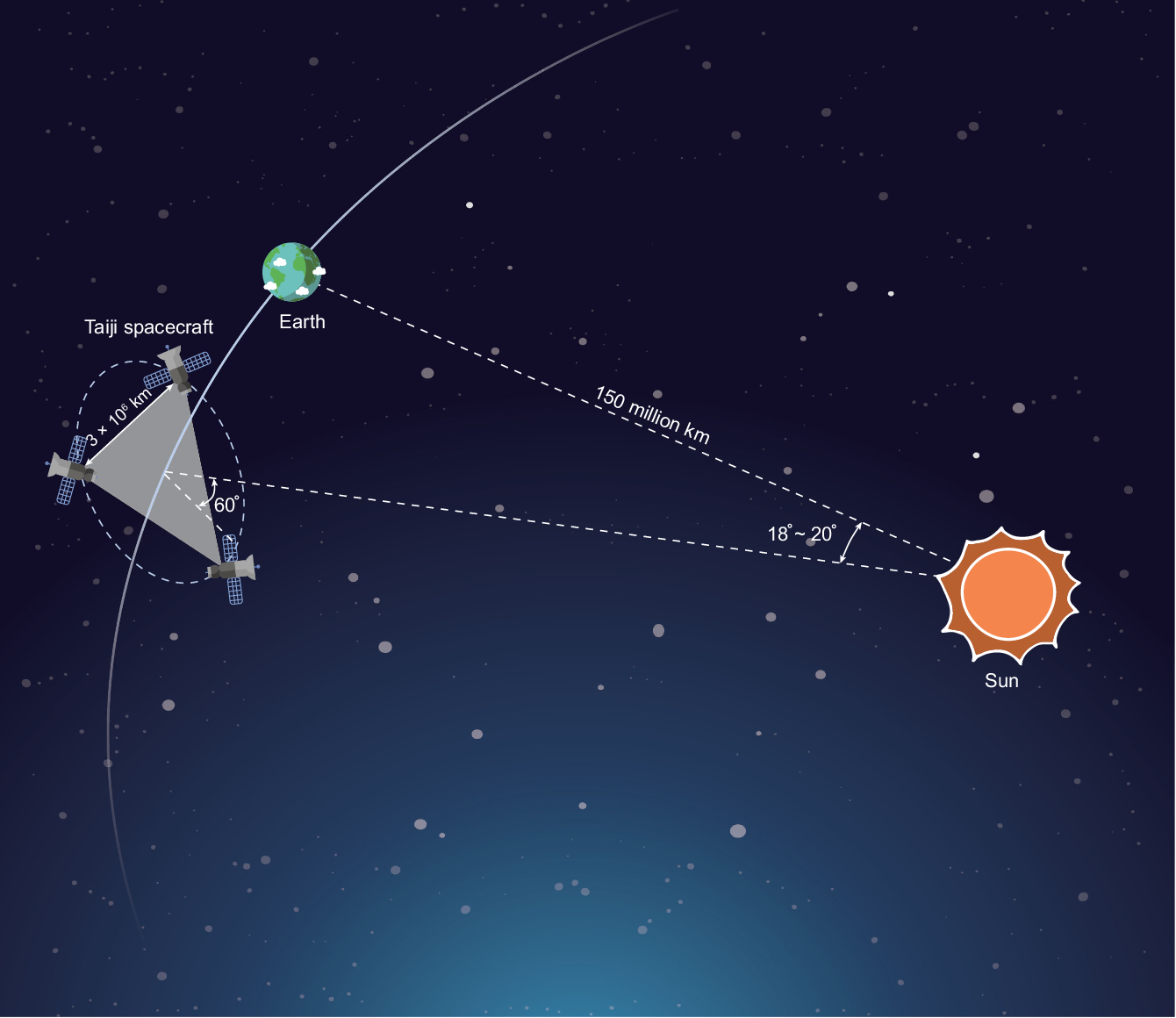
Project: Taiji program
M. Du, B. Liang, HW*, P. Xu, Z. Luo, Y. Wu*. SCPMA 67, 230412 (2024).
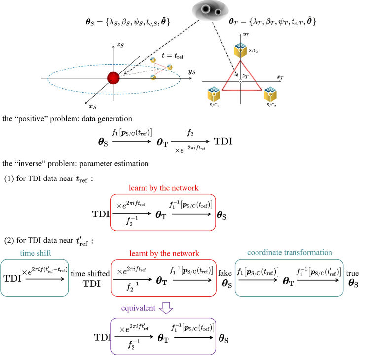
The top section of the illustration shows the solar system barycenter (SSB) and Taiji frames, with two black dashed arrows symbolizing not two separate GW signals, but rather indicating how the sky location and arrival time of the same GW signal take different values in these two frames.
The “positive” problem translates the SSB-frame parameters to their Taiji-frame counterparts via a time-dependent mapping \(f_1\), then to the TDI outputs through a time-independent mapping \(f_2\), and an exponential term.
TDI-A
These steps can be schematically summarized as:
where \(\mathcal{T}_\alpha^{A, E}(f)\) is often referred to as the transfer function.
M. Du, B. Liang, HW*, P. Xu, Z. Luo, Y. Wu*. SCPMA 67, 230412 (2024).
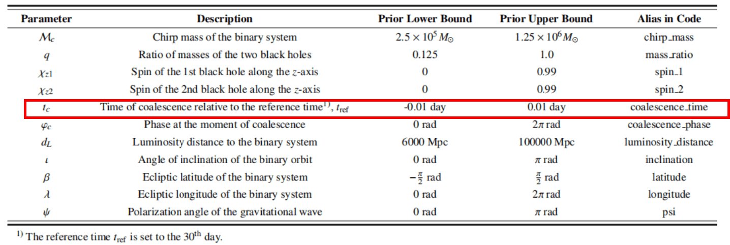
Consequently, even if the network has only learned the time-dependent relationship between \(\boldsymbol{\theta}_S\) and the TDI response at a specific tref (the 30th day in our case), with the aid of coordinate transformation, it has essentially learned the time-invariant mapping \(f_2\), and can be then generalized to make parameter estimation at any other reference time.
It is worth noting that our method relies on analytical orbits and
the time-independence of the coordinate transformation \(f_2\).
The top section of the illustration shows the solar system barycenter (SSB) and Taiji frames, with two black dashed arrows symbolizing not two separate GW signals, but rather indicating how the sky location and arrival time of the same GW signal take different values in these two frames.
The “positive” problem translates the SSB-frame parameters to their Taiji-frame counterparts via a time-dependent mapping \(f_1\), then to the TDI outputs through a time-independent mapping \(f_2\), and an exponential term.
1 year length
can infer at any other reference time
trained on the 30th day only
M. Du, B. Liang, HW*, P. Xu, Z. Luo, Y. Wu*. SCPMA 67, 230412 (2024).
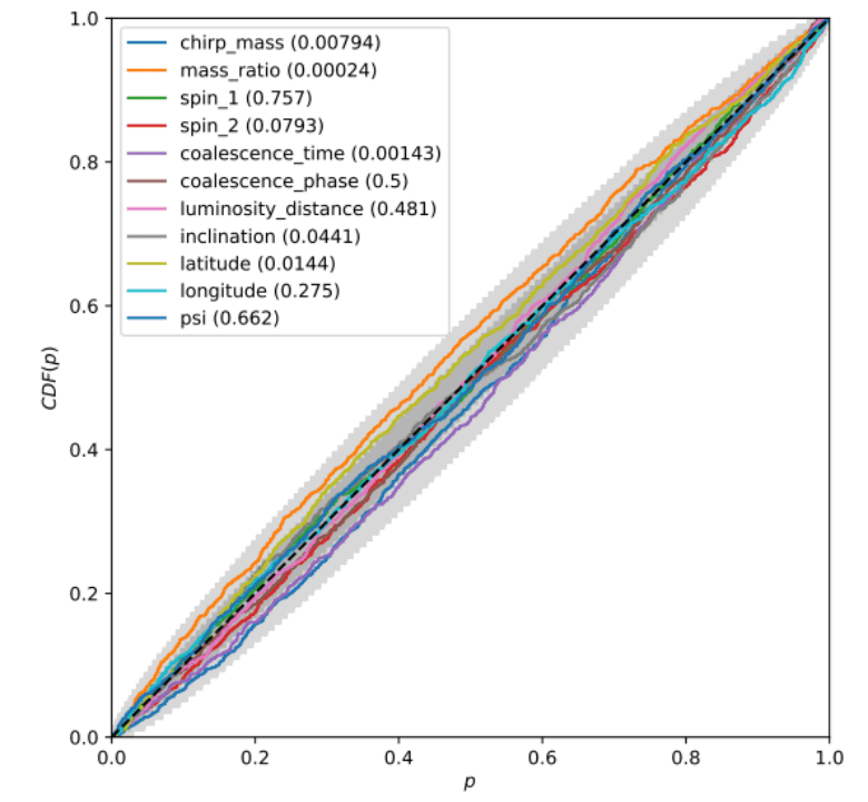
Methodology: Utilization of the Kolmogorov-Smirnov (KS) test to compare one-dimensional distributions generated by our algorithms, ensuring the accuracy of parameter estimation.
Empirical Validation: Conducted extensive testing on simulated signals, injecting 1000 waveforms from the prior with added confusion noise and varying reference times between 1 and 365 days.
Results: The tests assessed the frequency at which true parameters fell within certain confidence levels, confirming that our credible intervals are well-calibrated and reflect true confidence in the signal parameters.
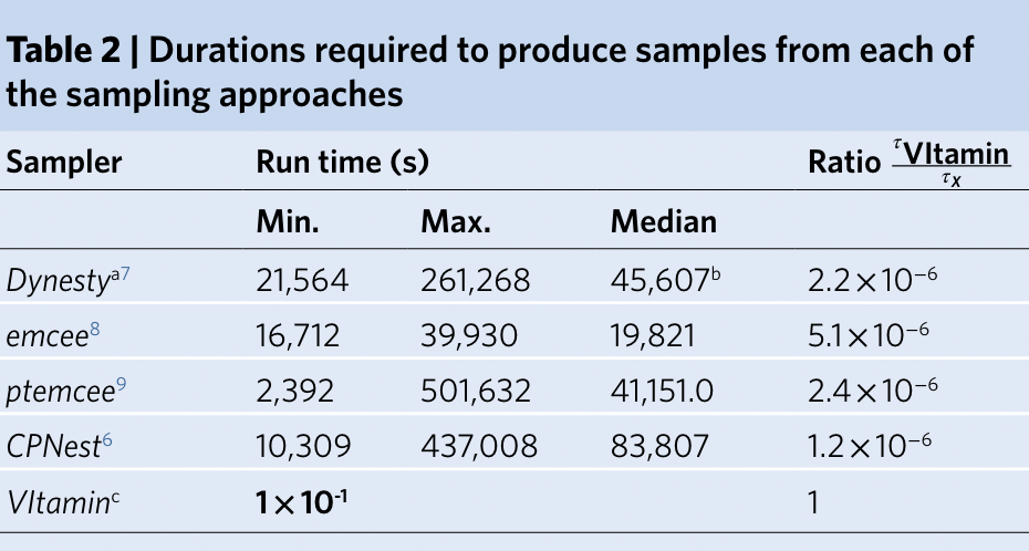
Computational performance
10000 posterior samples in 2.7 sec
M. Du, B. Liang, HW*, P. Xu, Z. Luo, Y. Wu*. SCPMA 67, 230412 (2024).
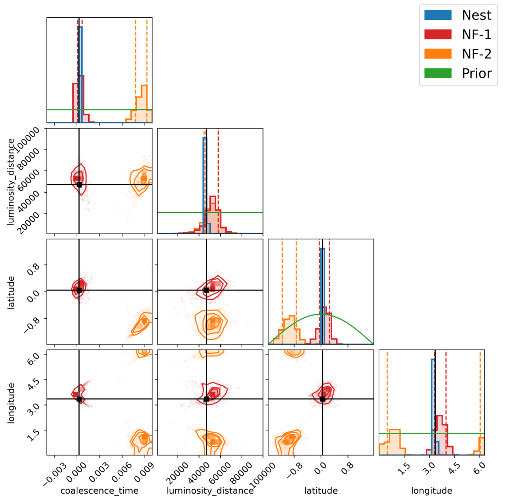
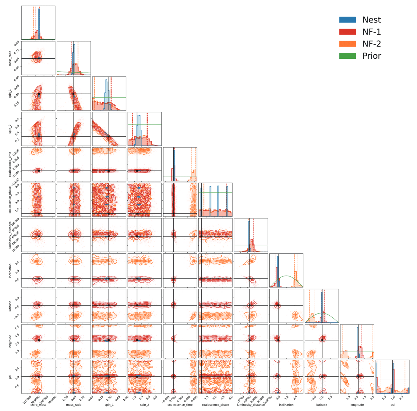
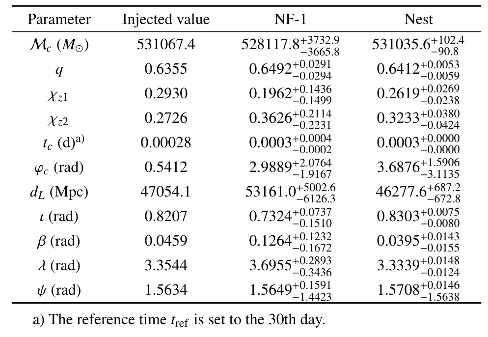
Overview of Findings: Nested sampling results indicate minimal expected multimodality in ecliptic coordinates. However, distinct peaks identified in the time of coalescence (\(t_c\)), labeled as NF-1 (dominant) and NF-2 (subdominant), highlight unique multimodal behavior.
(NF = Normalizing Flow model)
M. Du, B. Liang, HW*, P. Xu, Z. Luo, Y. Wu*. SCPMA 67, 230412 (2024).
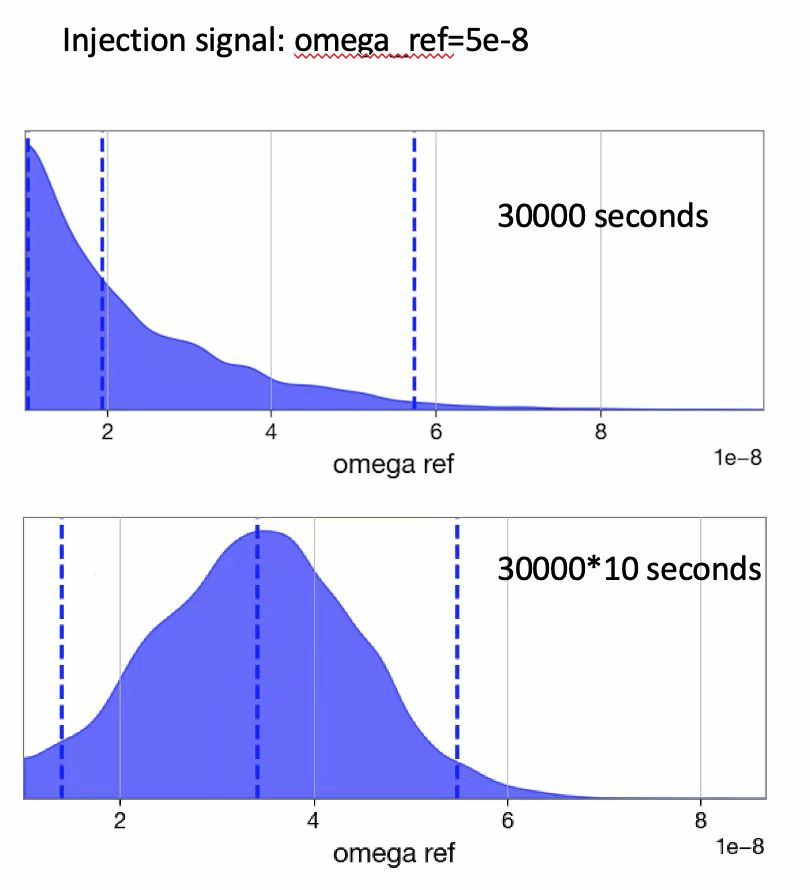
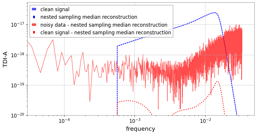
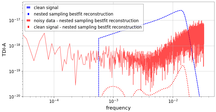
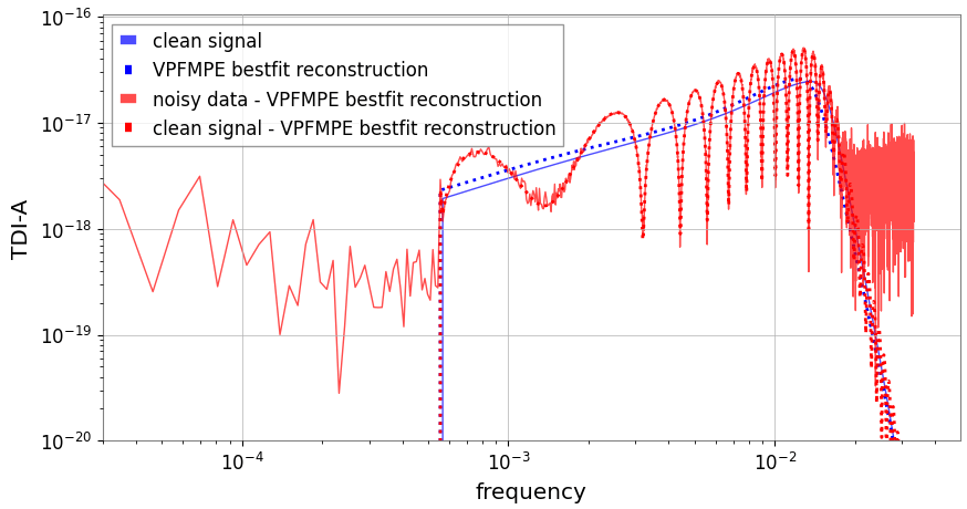
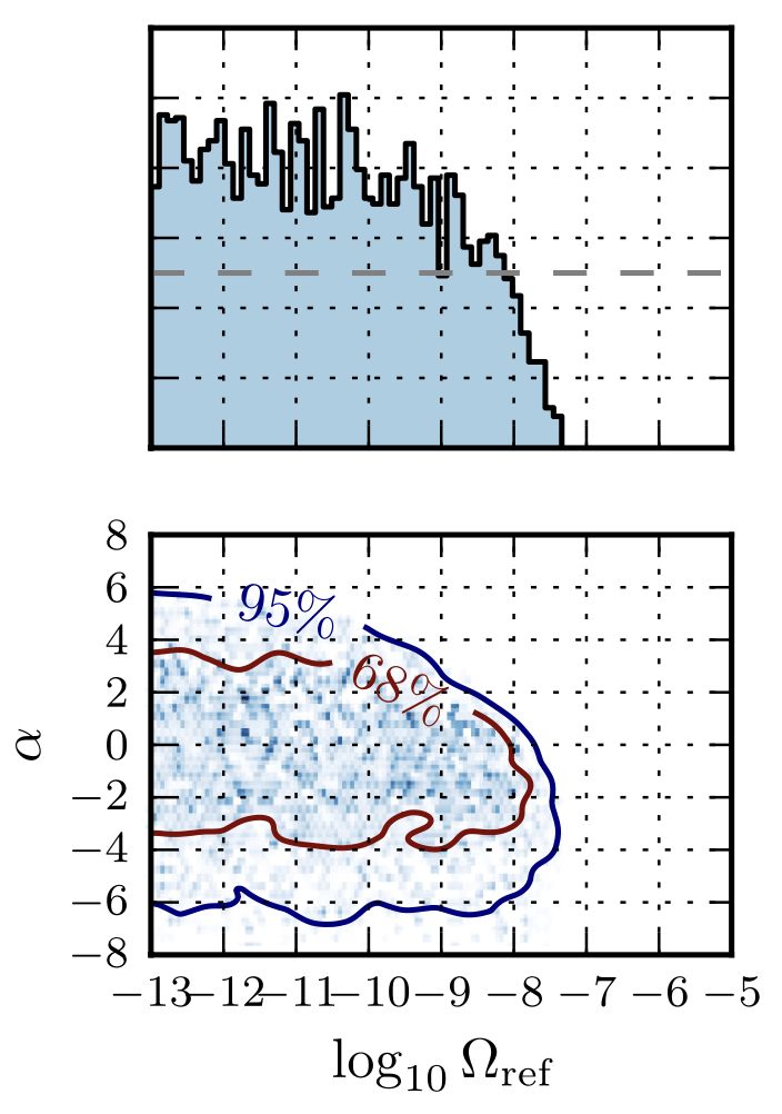
AI vs Classical Methods
Alfaidi & Messerger. arXiv:2402.04589
Our result (preliminary)
Menéndez-Vázquez A, et al. PRD 2021
PyGWB result
He Wang et al 2024 Mach. Learn.: Sci. Technol. 5 015046
Statistics
Statistics
AI vs Classical Methods
Calibration Analysis on Denoised / Residual Data
He Wang et al 2024 Mach. Learn.: Sci. Technol. 5 015046
M. Du, B. Liang, HW*, P. Xu, Z. Luo, Y. Wu*. SCPMA 67, 230412 (2024).
for _ in range(num_of_audiences):
    print('Thank you for your attention! 🙏')
This silde: https://slides.com/iphysresearch/2024august_uoa
Calibration Analysis on Denoised / Residual Data
He Wang et al 2024 Mach. Learn.: Sci. Technol. 5 015046
M. Du, B. Liang, HW*, P. Xu, Z. Luo, Y. Wu*. SCPMA 67, 230412 (2024).
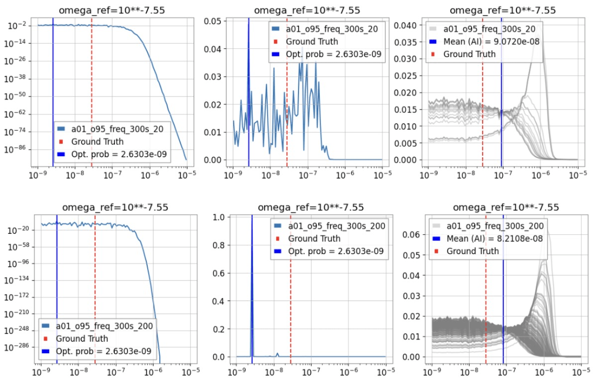
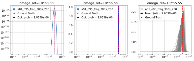
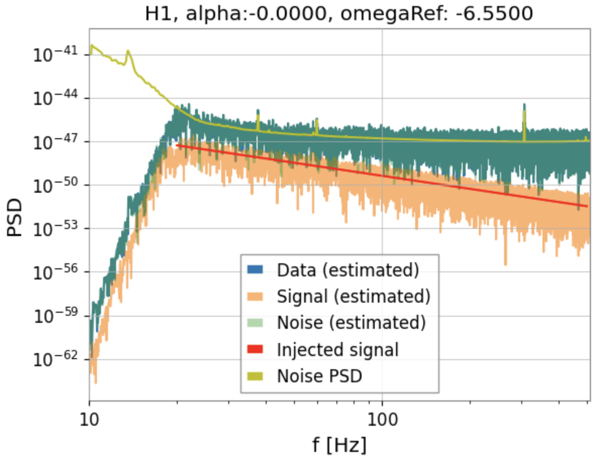
Exploring Stochastic Gravitational Wave Background with AI
Our result (preliminary)
Exploring Stochastic Gravitational Wave Background with AI
Abbott R, et al. PRD 104, 2 (2021): 022004.
PyGWB result
Our result (preliminary)
By He Wang
August 2 at 3pm NZ time, @University of Auckland