


He Wang PRO
Knowledge increases by sharing but not by saving.
2026/05/09 @内蒙古大学
Upcoming challenges such as MLGWSC2, currently at the proposal stage, provide a new testbed for exploring machine-learning–based approaches to gravitational-wave analysis. In this flash talk, I briefly introduce my core ideas and experience using evolutionary algorithms, Evo-MCTS, and reinforcement learning as adaptive search and optimization tools. I outline key methodological insights and discuss how these ideas may inform future GW analysis tasks, including potential applications to LISA.
才翻到上面看到有人现场拍照 [破涕为笑],随手分享一下
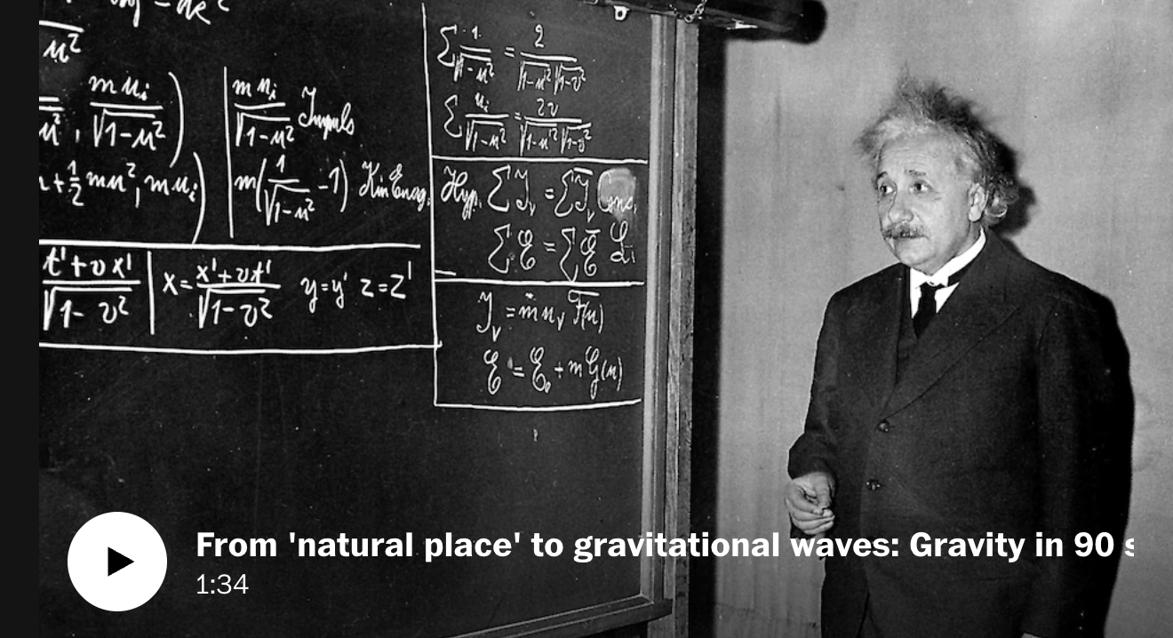
引力波是时空的涟漪。
大物体的引力扭曲空间和时间,或称为“时空”,就像保龄球在弹跳床上滚动时改变其形状一样。较小的物体因此会以不同的方式移动——就像弹跳床上朝向保龄球大小的凹陷螺旋而去的弹珠,而不是坐在平坦的表面上。
爱因斯坦于1916年提出广义相对论,并预言了引力波的存在
引力波是广义相对论中的一种强场效应
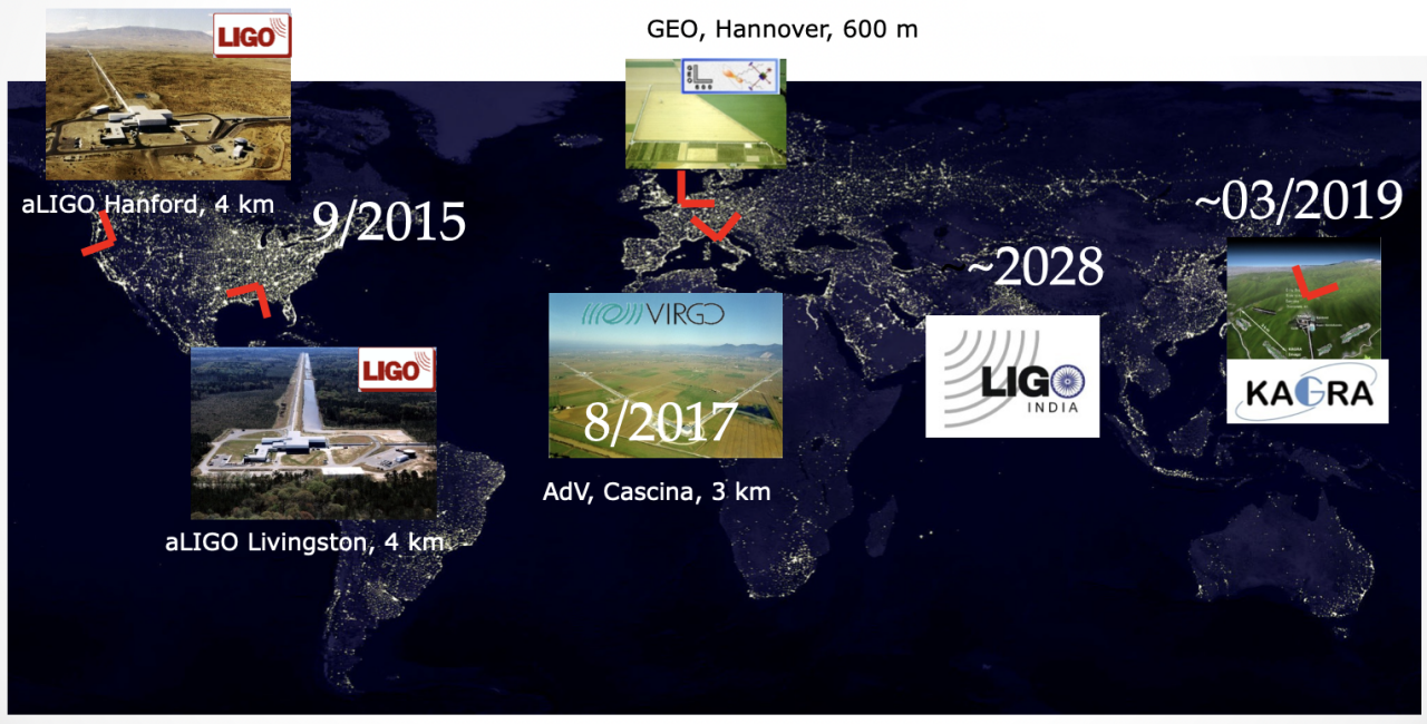
2015年:首次实验探测到双黑洞并合引力波
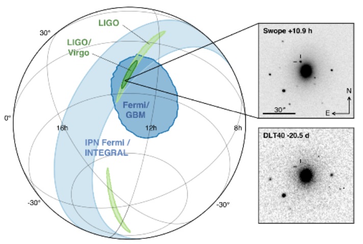
2017年:首次双中子星多信使探测,开启多信使天文学时代
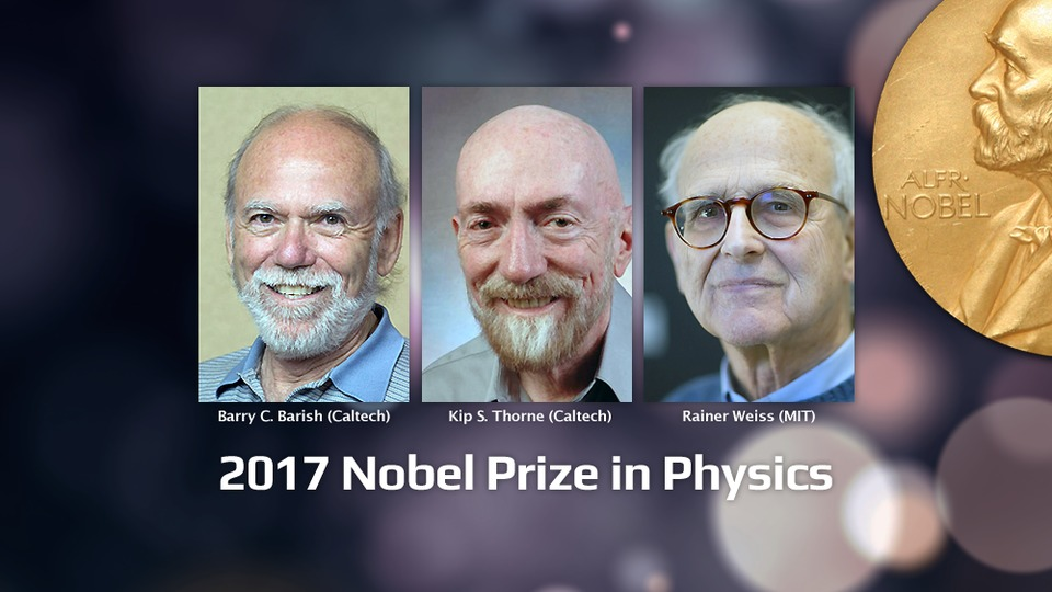
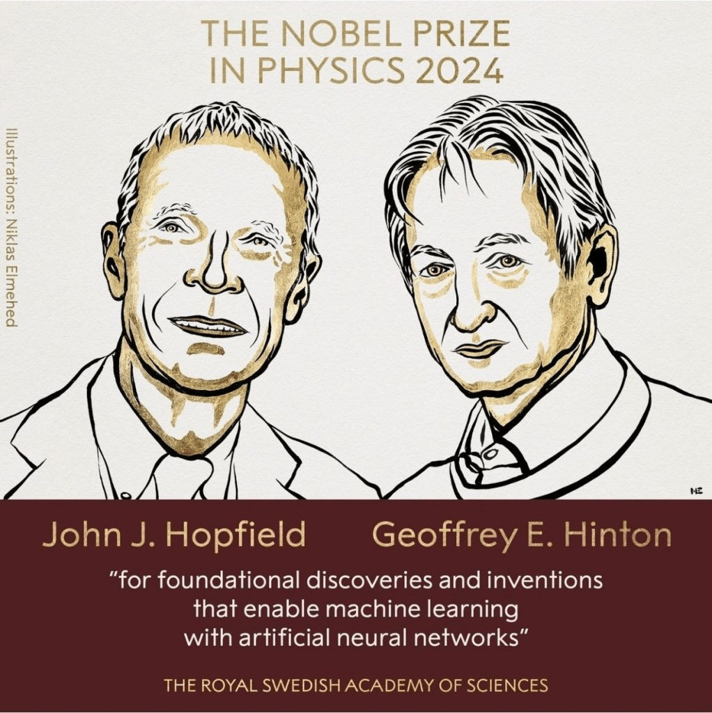
2017年:引力波探测成果被授予诺贝尔物理学奖
至今:发现了超过 90 个引力波事件
2024年:中国科学院大学加入地面引力波实验LIGO科学合作组织,成为LIGO目前在中国大陆地区的第二家成员单位。
未来规划:
2024-2025年:有希望探测到更多不同类型的引力波事件
空间引力波探测计划 (LISA/Taiji/Tianqin) + XG (CE/ET)
...
LIGO-VIRGO-KAGRA network
Gravitational waves generated by binary black holes system
GW detector
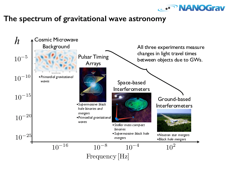
引力波探测打开了探索宇宙的新窗口
不同波源,频率跨越 20 个数量级,不同探测器
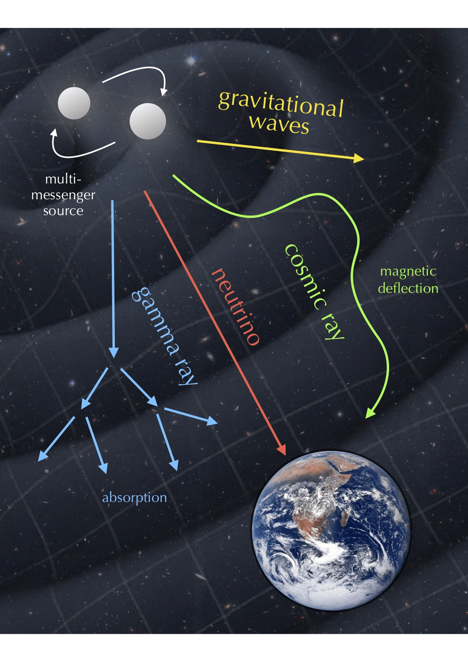
四种系外信使包括:电磁辐射、引力波、中微子,以及宇宙射线。
多信使天文学
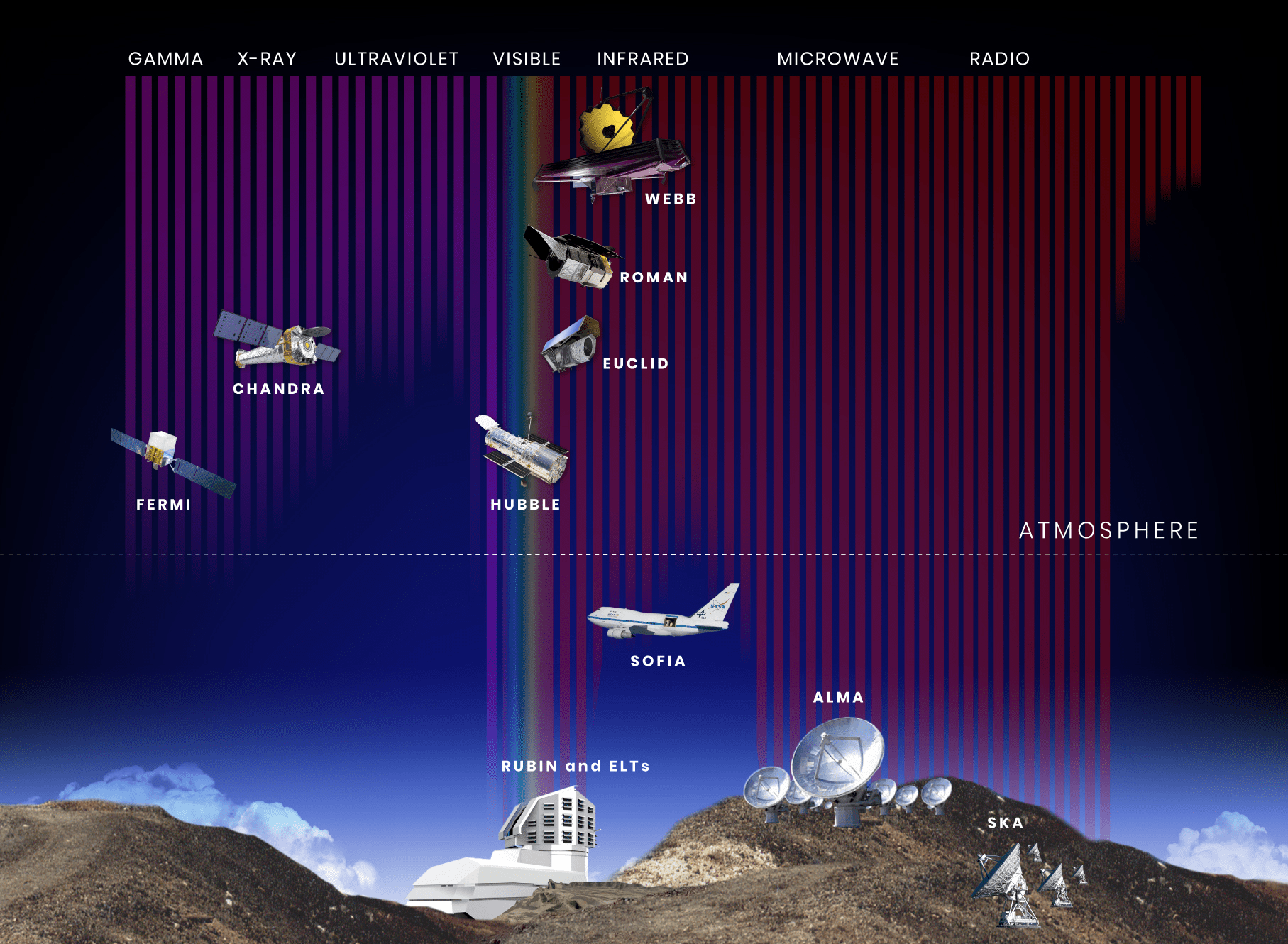
“电磁波天文学”
DOI:10.1063/1.1629411
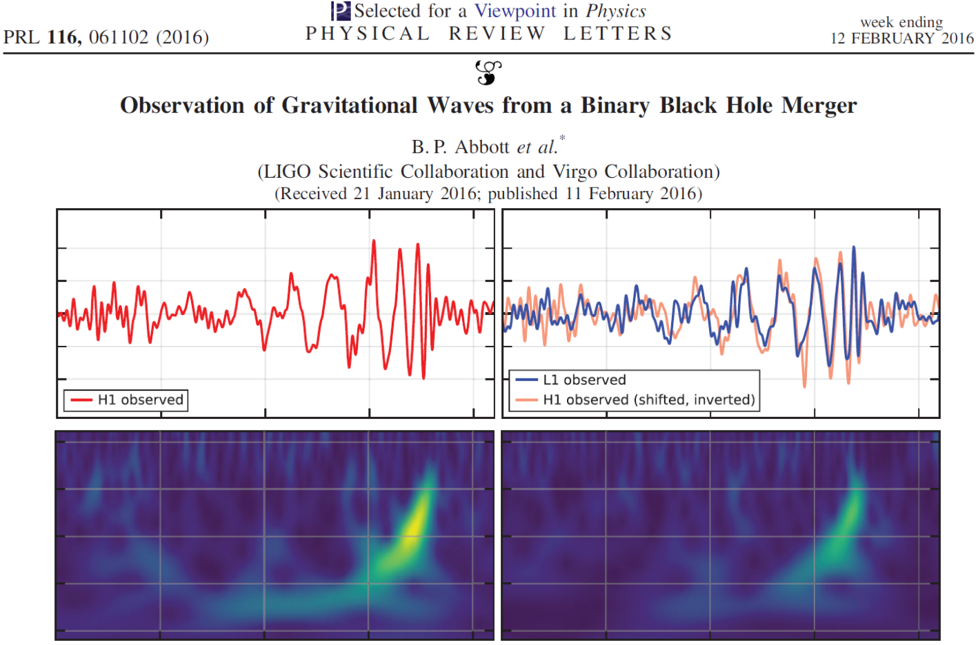
The first GW event of GW150914
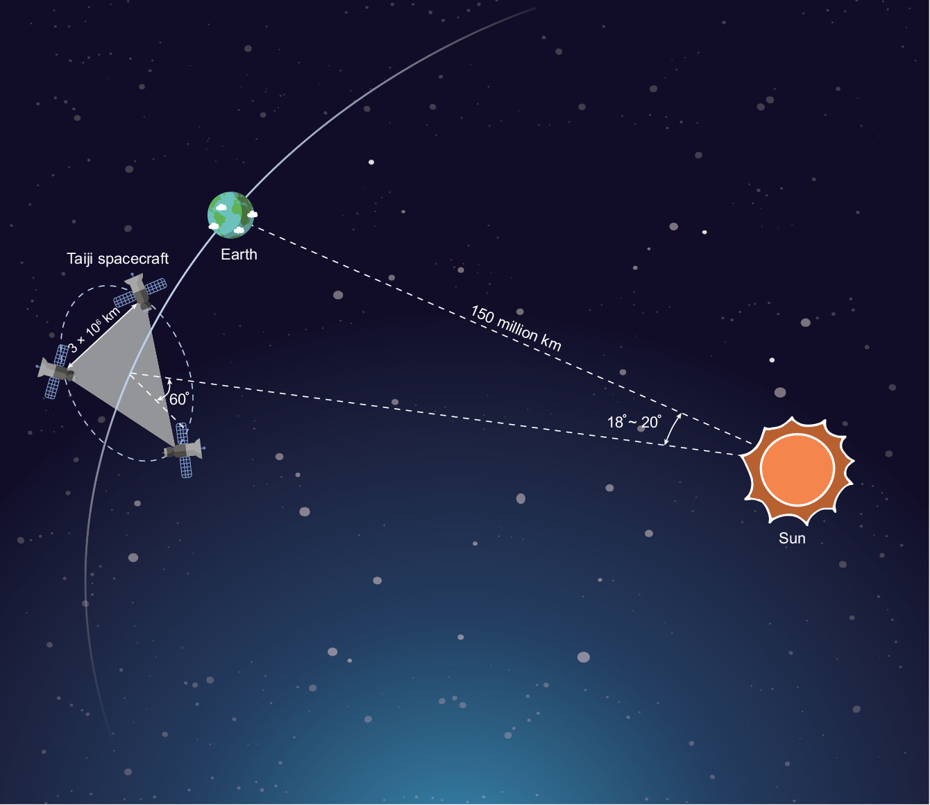
LISA / Taiji project
LIGO-VIRGO-KAGRA
GW Data Characteristics
LIGO-VIRGO-KAGRA
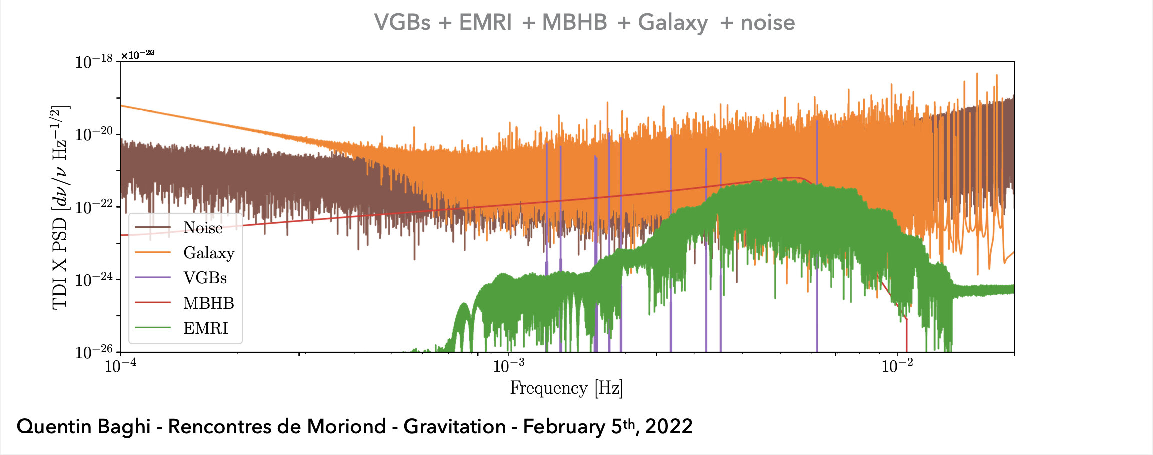
LISA Project
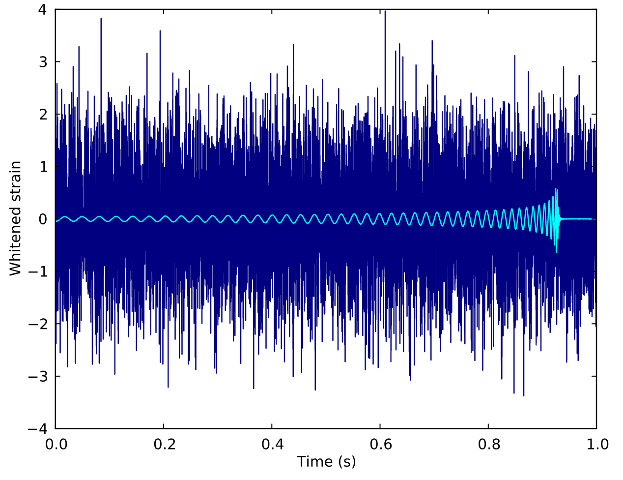
Noise: non-Gaussian and non-stationary
Signal challenges:
(Earth-based) A low signal-to-noise ratio (SNR) which is typically about 1/100 of the noise amplitude (-60 dB).
(Space-based) A superposition of all GW signals (e.g.: 104 of GBs, 10~102 of SMBHs, and 10~103 of EMRIs, etc.) received during the mission's observational run.
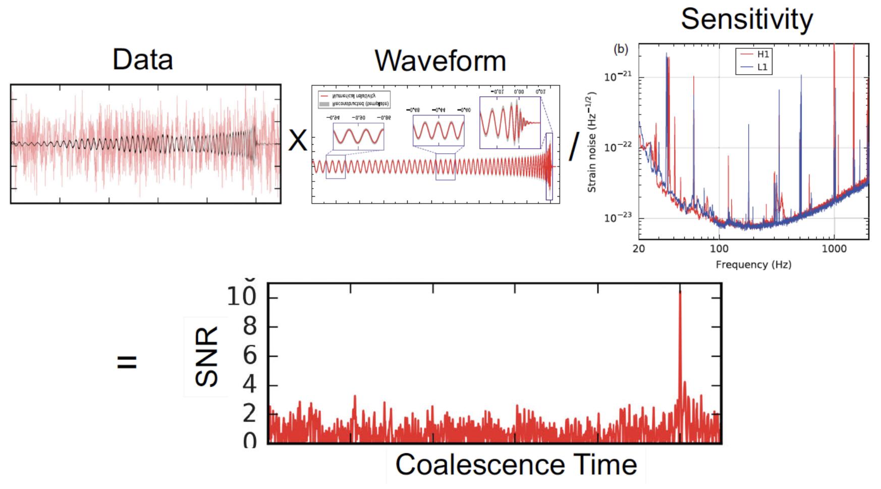
Matched Filtering Techniques (匹配滤波方法)
In Gaussian and stationary noise environments, the optimal linear algorithm for extracting weak signals
Statistical Approaches
Frequentist Testing:
Bayesian Testing:
GW Data Characteristics
LIGO-VIRGO-KAGRA
LISA Project
Noise: non-Gaussian and non-stationary
Signal challenges:
(Earth-based) A low signal-to-noise ratio (SNR) which is typically about 1/100 of the noise amplitude (-60 dB).
(Space-based) A superposition of all GW signals (e.g.: 104 of GBs, 10~102 of SMBHs, and 10~103 of EMRIs, etc.) received during the mission's observational run.
Matched Filtering Techniques (匹配滤波方法)
In Gaussian and stationary noise environments, the optimal linear algorithm for extracting weak signals
Statistical Approaches
Frequentist Testing:
Bayesian Testing:
线性滤波器
输入序列
输出序列
脉冲响应函数:
Digital Signal Processing
地基引力波探测科学数据的特点
噪声特点:非高斯 + 非稳态
信号特点:信噪比低 (约噪声幅度的1/100,约 -60dB )
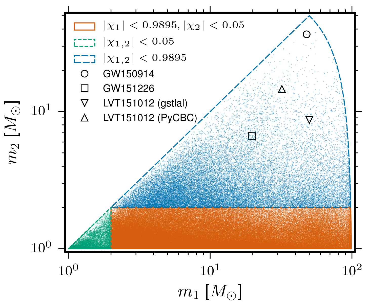
波形模板库的局限性
需要大量的精确波形模板以确保无遗漏,至少百万数量级
受限于已知引力理论预言的波形模板,难以搜寻超越经典广相引力理论 的引力波信号
多信使天文学的兴起 + 引力波探测技术的进步
低(负)延迟 的引力波信号搜寻
海量的 累积数据和 成批的 引力波事件,有待高效的仔细分析
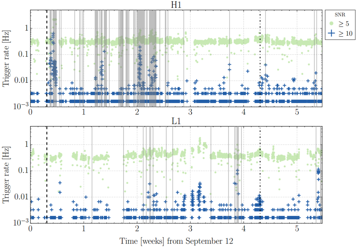
真实引力波数据的非高斯性
O1 观测运行时用的波形模板库
在 GW170817 事件后 1.74\(\pm\)0.05s 的伽玛暴 GRB 170817A
AlphaGo
围棋机器人
AlphaTensor
发现矩阵算法
AlphaFold
蛋白质结构预测
验证数学猜想
AlphaGo
围棋机器人
AlphaTensor
发现矩阵算法
AlphaFold
蛋白质结构预测
验证数学猜想
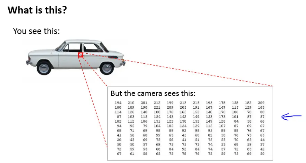
Uncovering the "black box" to reveal how AI actually works
Core Insight from Computer Vision
Performance Analysis
Pioneering Research Publications
PRL, 2018, 120(14): 141103.
PRD, 2018, 97(4): 044039.
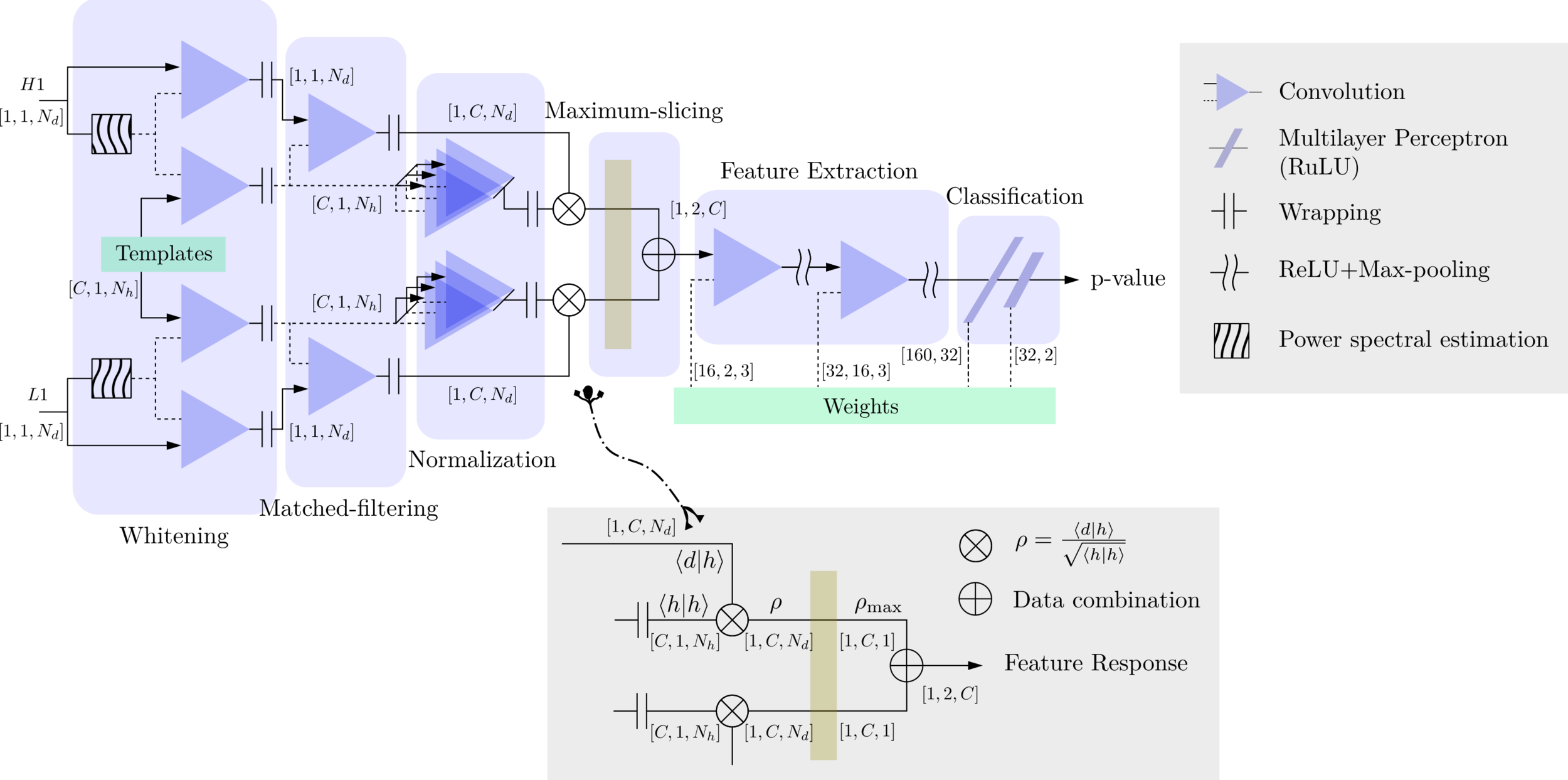
Matched-filtering Convolutional Neural Network (MFCNN)
HW, SC Wu, ZJ CAO, et al. PRD 101, 10 (2020): 104003
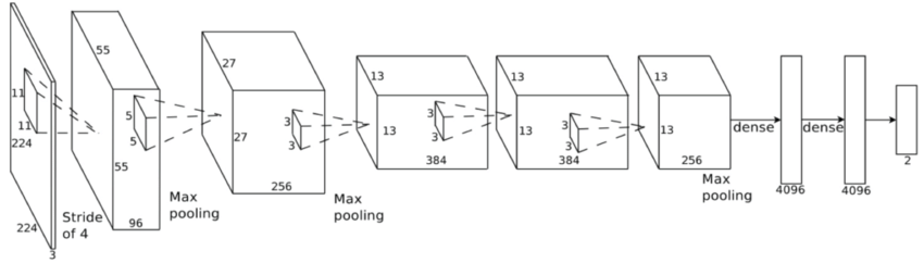
Convolutional Neural Network (ConvNet or CNN)
feature extraction
classifier
>> Is it matched-filtering ?
>> Wait, It can be matched-filtering!
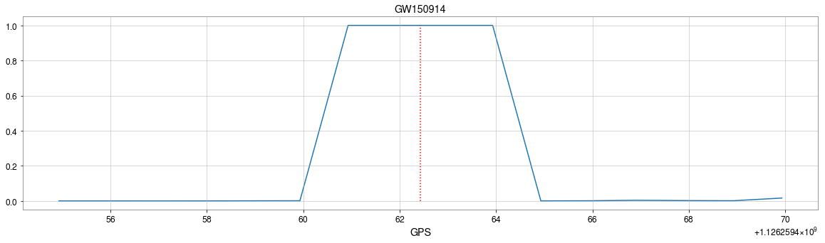
GW150914
GW150914
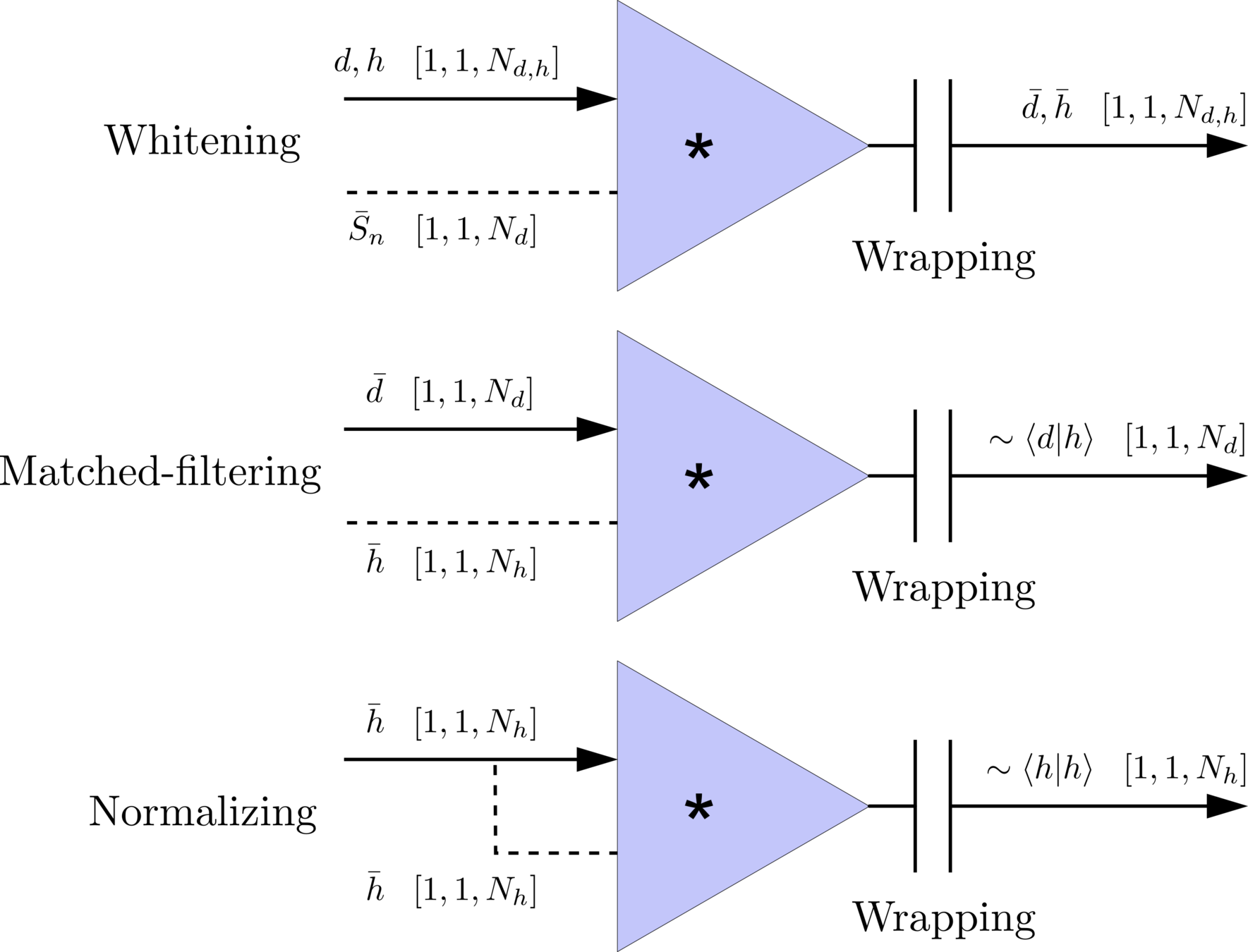
Transform matched-filtering method from frequency domain to time domain.
The square of matched-filtering SNR for a given data \(d(t) = n(t)+h(t)\):
\(S_n(|f|)\) is the one-sided average PSD of \(d(t)\)
where
Deep Learning Framework
Time Domain
(matched-filtering)
(normalizing)
(whitening)
Frequency Domain
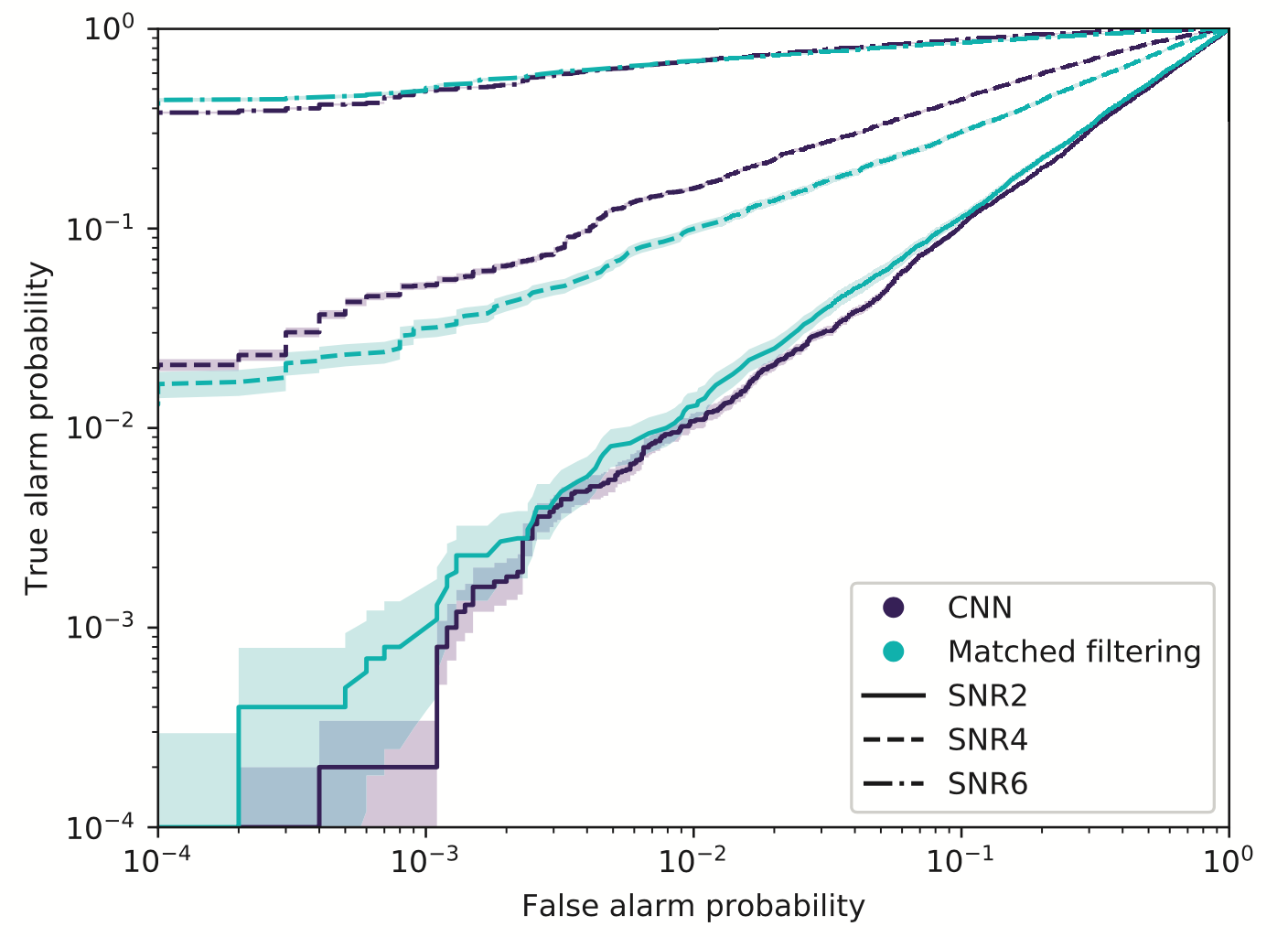
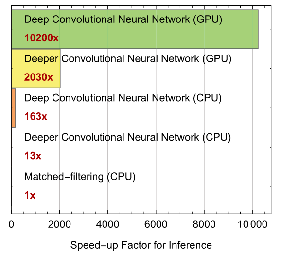
Benchmark Results
Publications
Key Findings
Note on Benchmark Limitations:
Outperforming PyCBC doesn't conclusively prove that matched filtering is inferior to AI methods. This is both because the dataset represents a specific distribution and because PyCBC settings could be further optimized for this particular benchmark.
arXiv:2501.13846 [gr-qc]
Phys. Rev. D 107, 023021 (2023)
B. P. Abbott et al. (LIGO-Virgo), PRD 100, 104036 (2019).
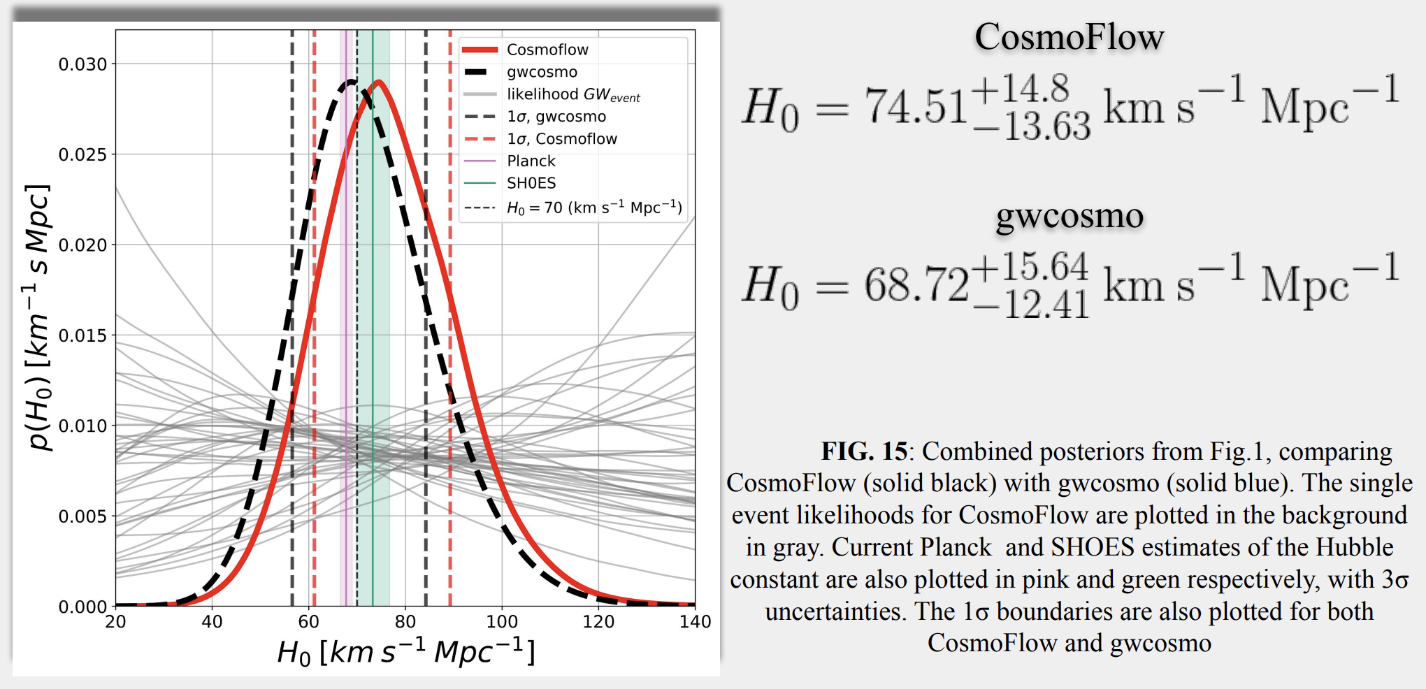
Yu-Xin Wang, Xiaotong Wei, Chun-Yue Li, Tian-Yang Sun, Shang-Jie Jin, He Wang*, Jing-Lei Cui, Jing-Fei Zhang, and Xin Zhang*. arXiv:2410.20129. PRD (2025)
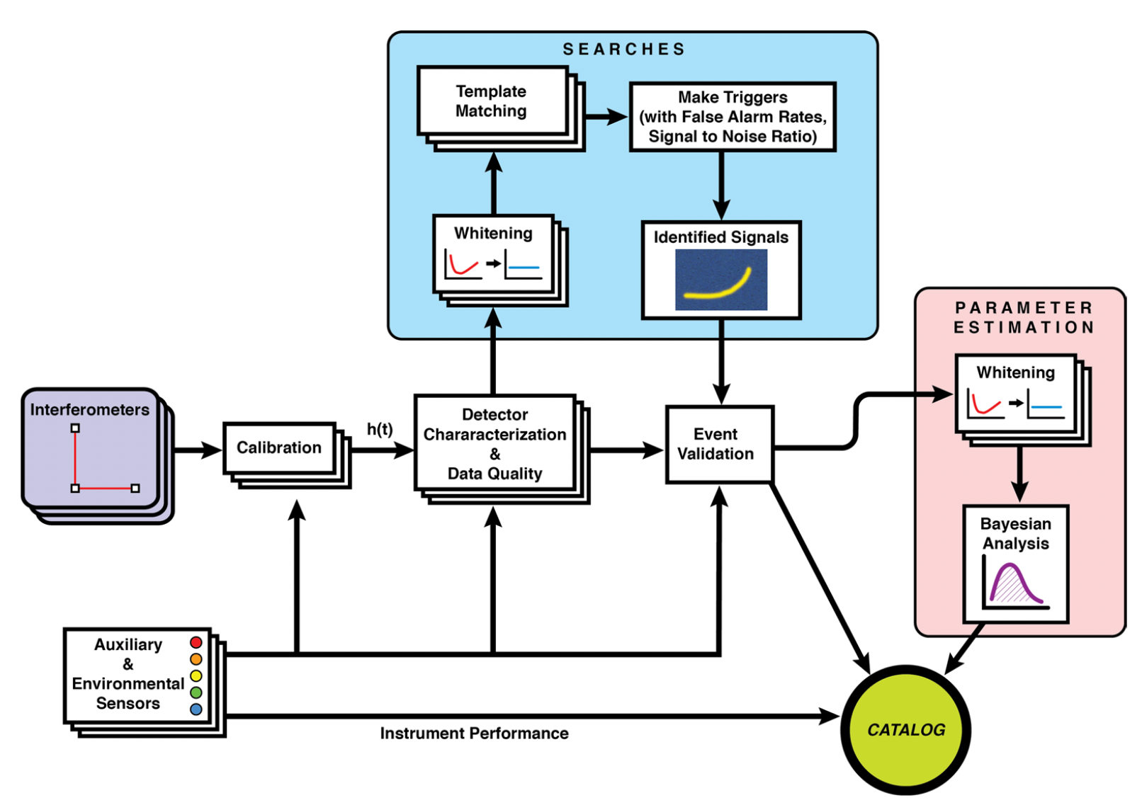
Bayesian statistics
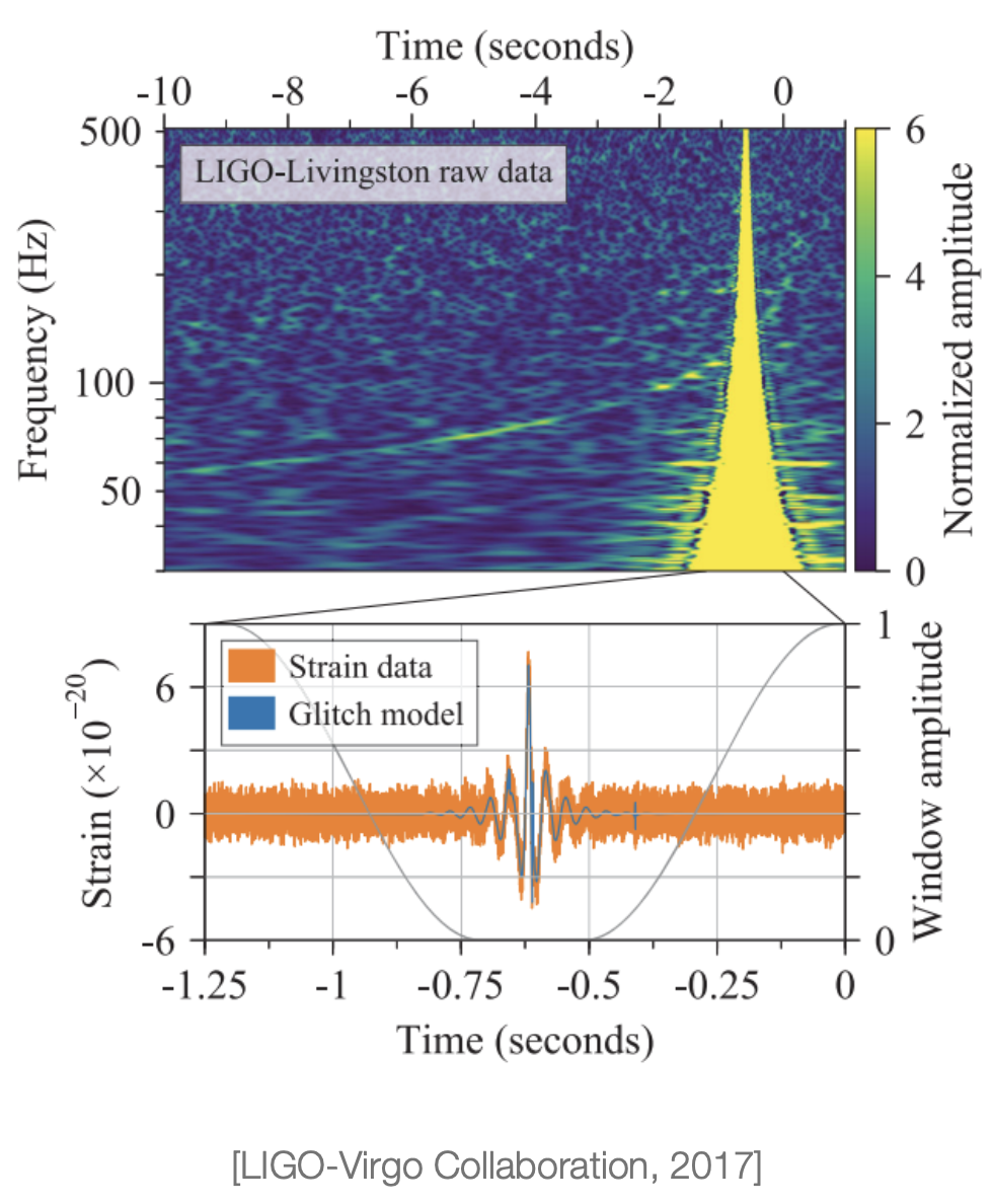
Data quality improvement
Credit: Marco Cavaglià
LIGO-Virgo data processing
GW searches
Astrophsical interpretation of GW sources
Credit: Marco Cavaglià
Nature Physics 18, 1 (2022) 112–17
PRL 127, 24 (2021) 241103.
PRL 130, 17 (2023) 171403.
HW, et al. Big Data Mining and Analytics 5, 1 (2021) 53–63.
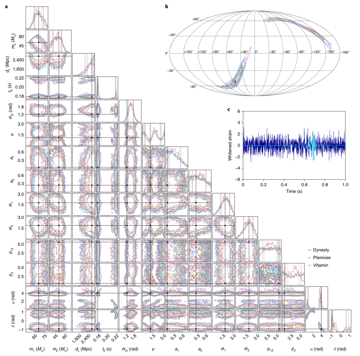
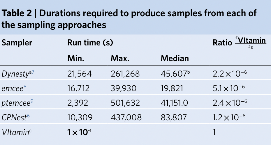
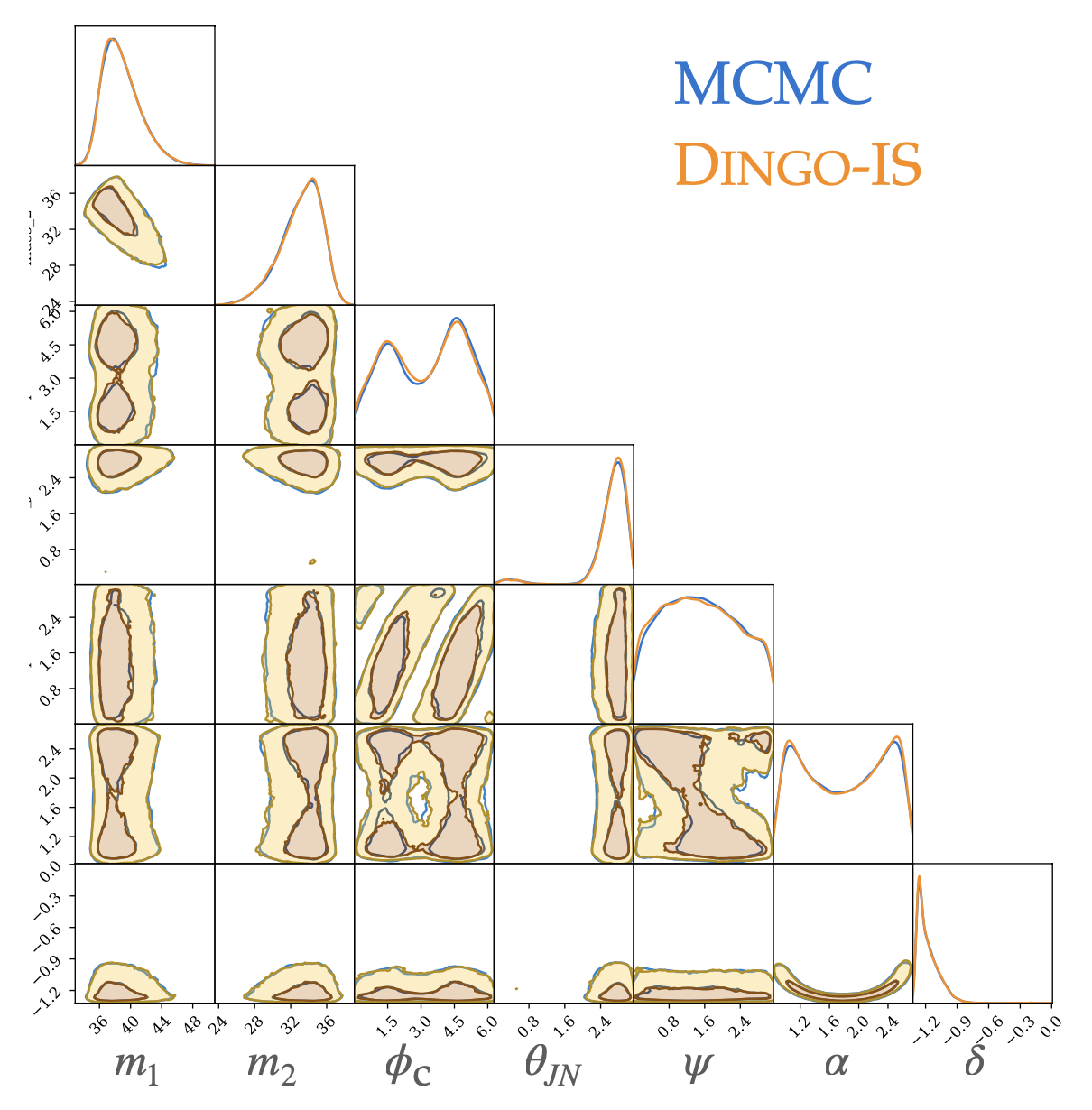
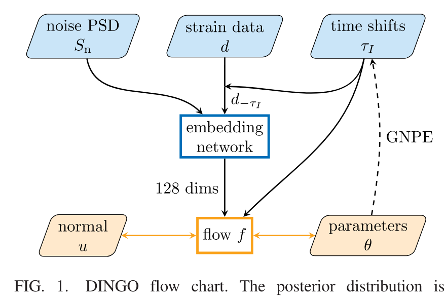
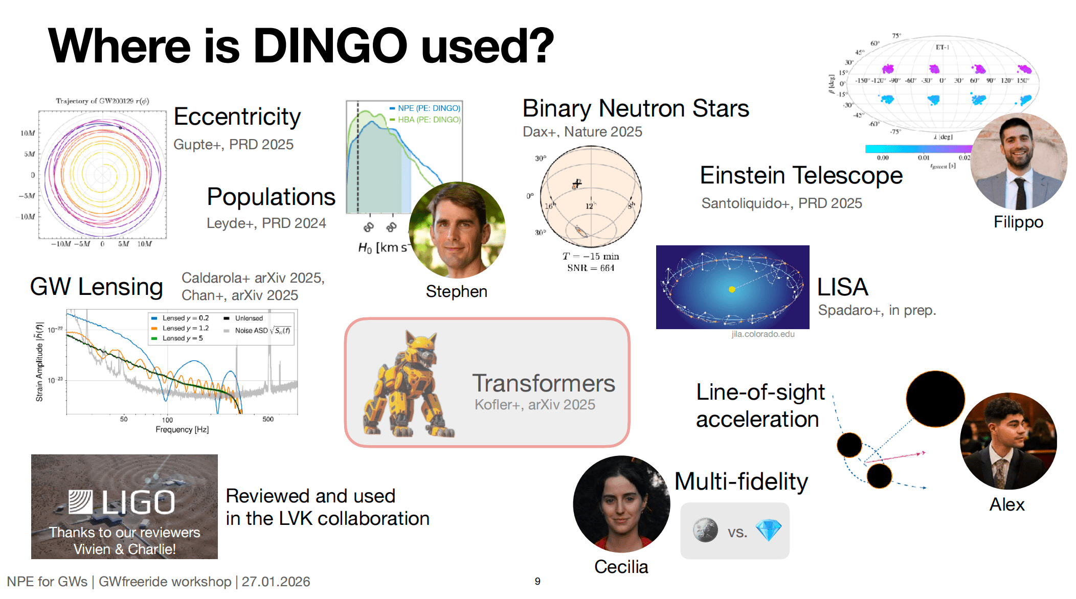
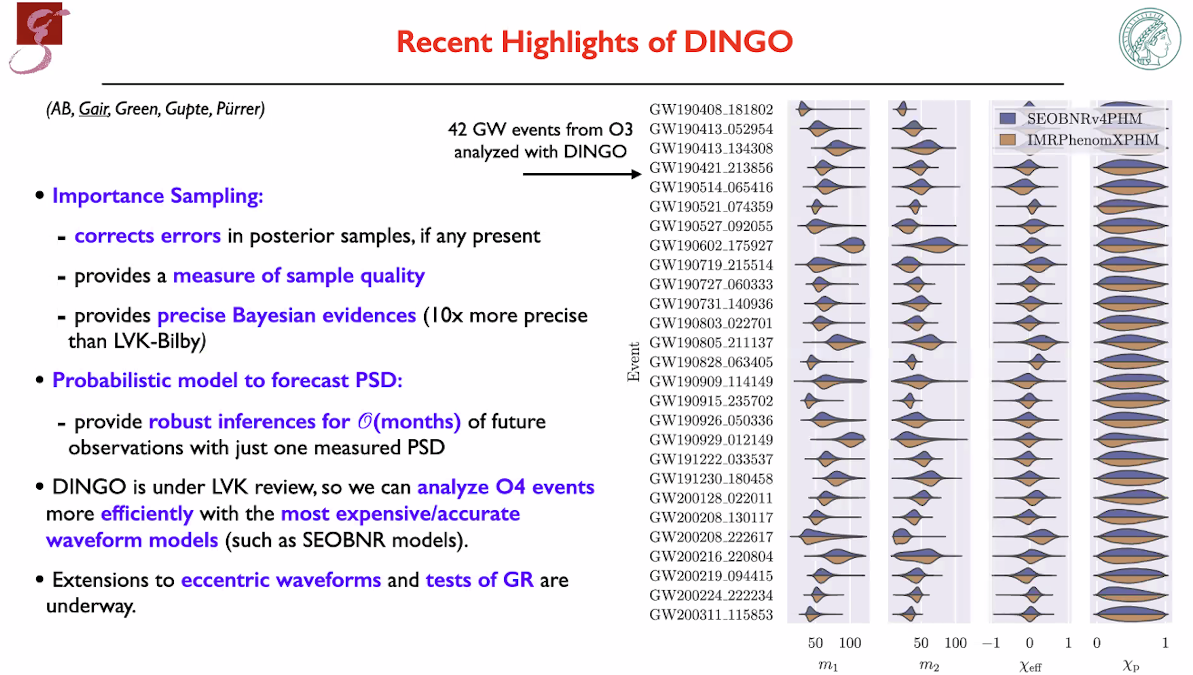
進撃の DINGO in GW inference area.
2002.07656: 5D toy model [1] (PRD)
2008.03312: 15D binary black hole inference [1] (MLST)
2106.12594: Amortized inference and group-equivariant neural posterior estimation [2] (PRL)
2111.13139: Group-equivariant neural posterior estimation [2] (ICLR 2022)
2210.05686: +Importance sampling [2] (PRL)
2211.08801: Noise forecasting [2] (PRD)
2311.12093: Population studies [2] (PRD)
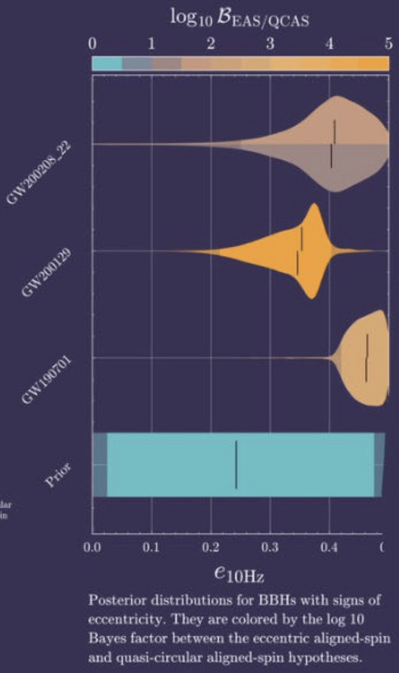
2404.14286: Find evidence for eccentric binaries. [2] (PRD)
2407.09602: BNS inference [2] (Nature)
2512.02968: +Transformer, (Dingo-T1) [3] (?)
2603.20431: For LISA [4] (?)
https://github.com/dingo-gw/dingo (2023.03)
https://github.com/dingo-gw/dingo-T1 (2025.11)
https://github.com/AliSword/dingo-lisa (2026.04)
https://github.com/stephengreen/gw-school-corfu-2023 (Tutorial)
https://github.com/annalena-k/tutorial-dingo-introduction (Tutorial)
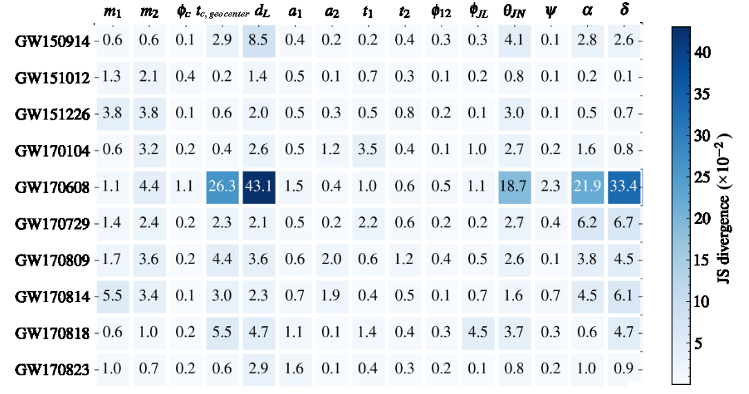
Parameter Estimation Challenges with AI Models:
Phys. Rev. D 112 (2025) 104045
Phys. Rev. D 109, 123547 (2024)
PRD 108, 4 (2023): 044029.
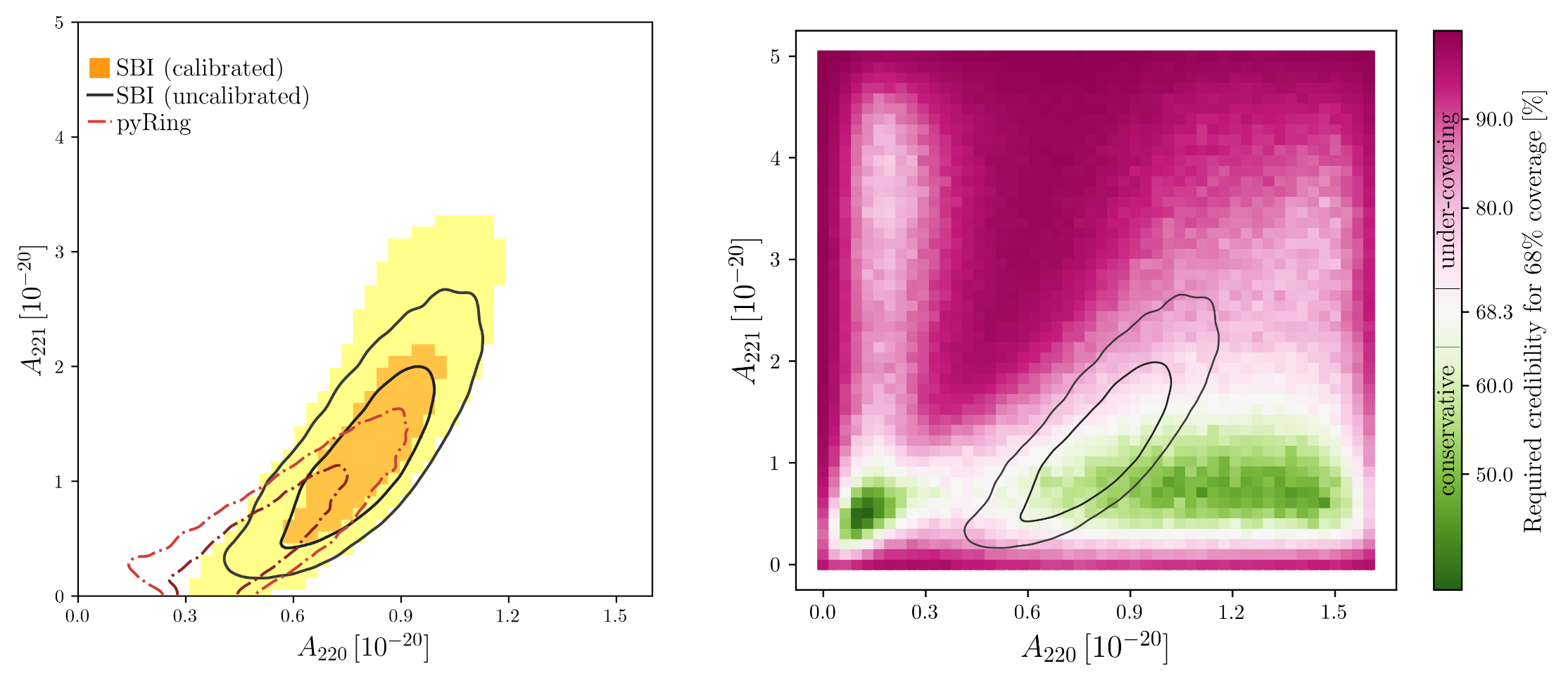
Neural Posterior Estimation with Guaranteed Exact Coverage: The Ringdown of GW150914
Train
nflow
Train
nflow
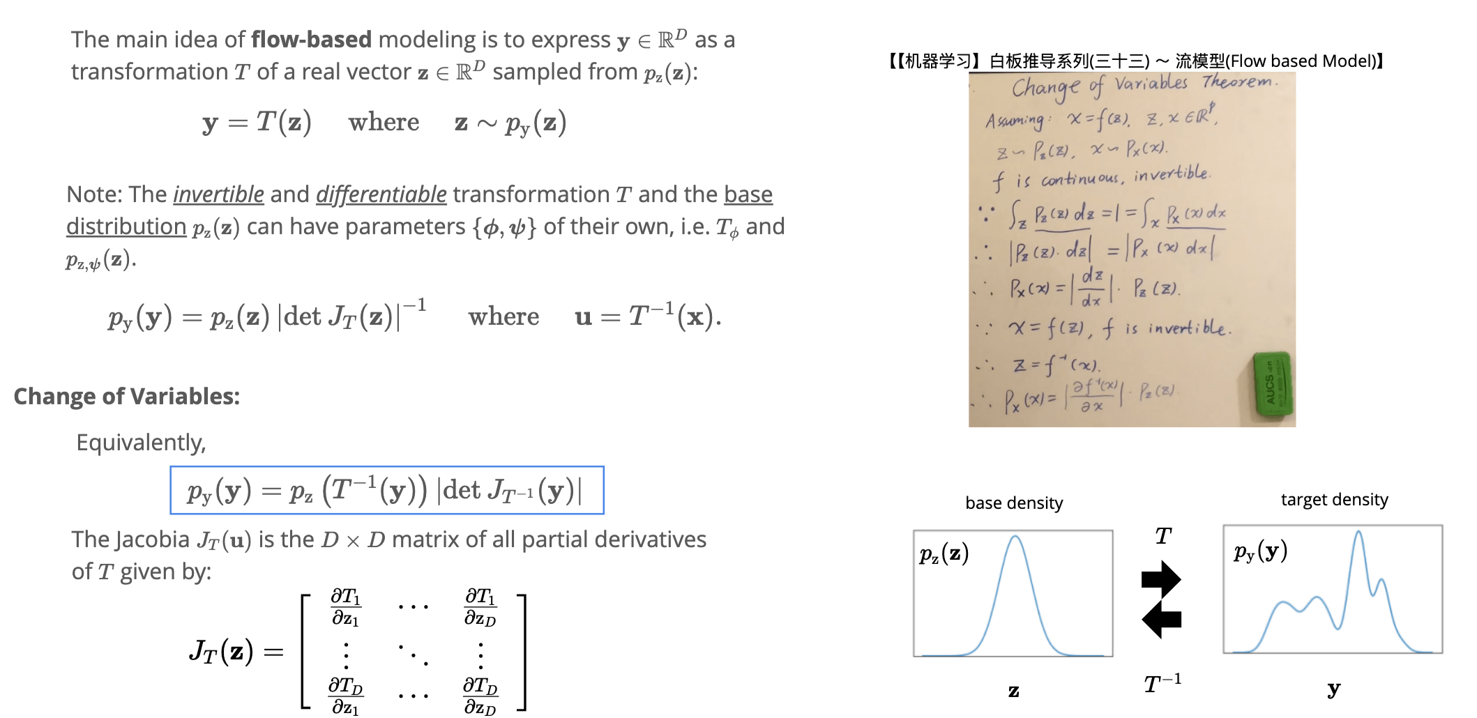
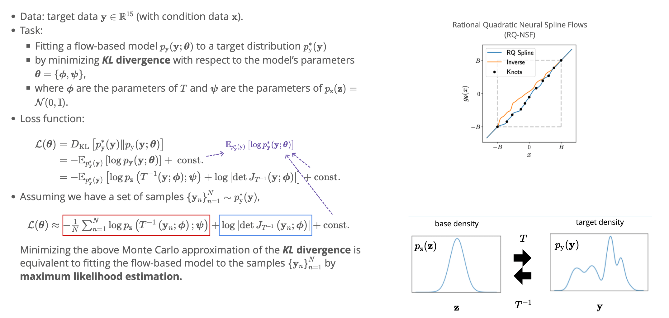
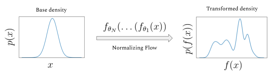
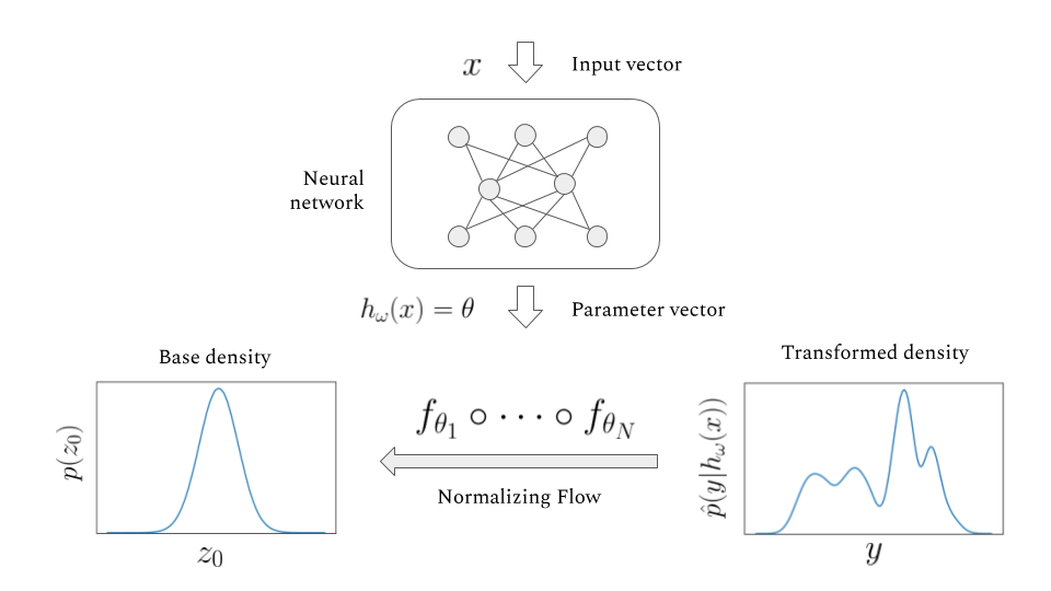
归一化流模型示意图
Test
nflow
base density
target density
Uncovering the "black box" to reveal how LLM actually works
HW, LZ. arXiv:2508.03661 [cs.AI]
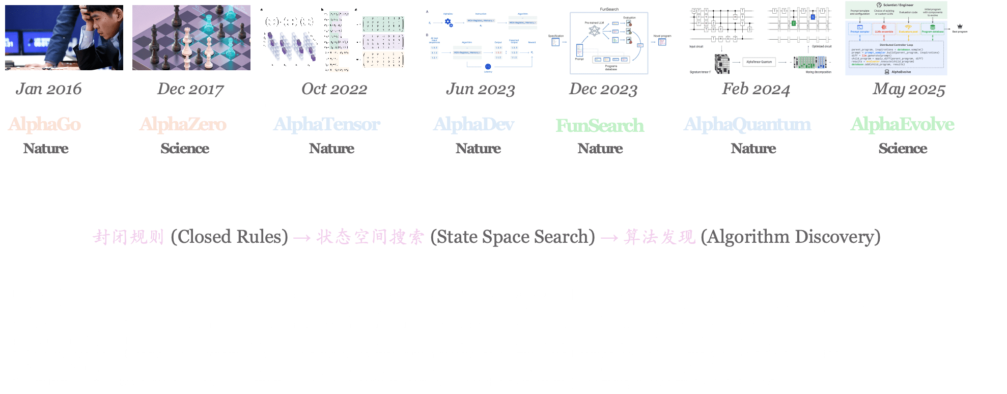
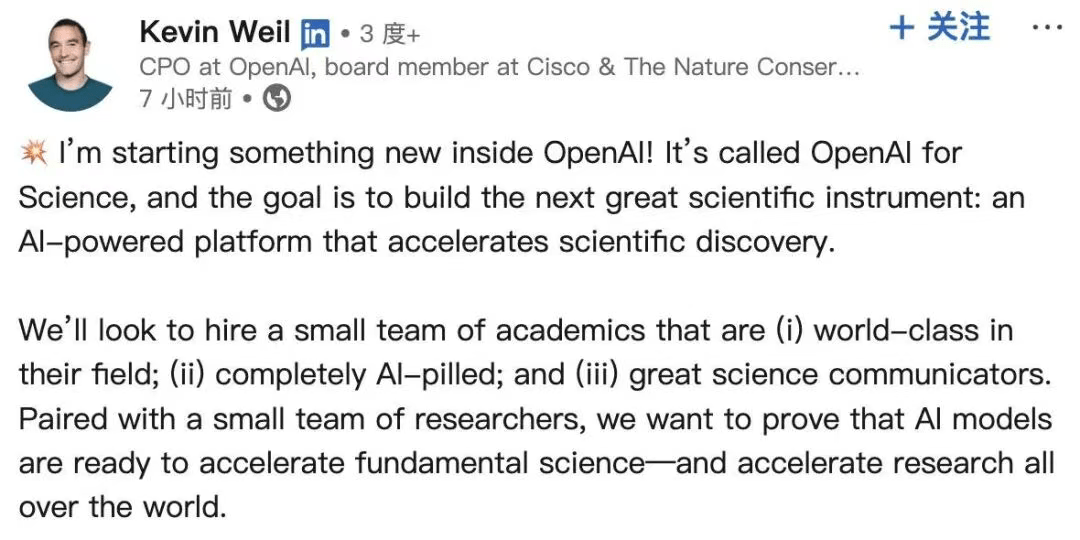
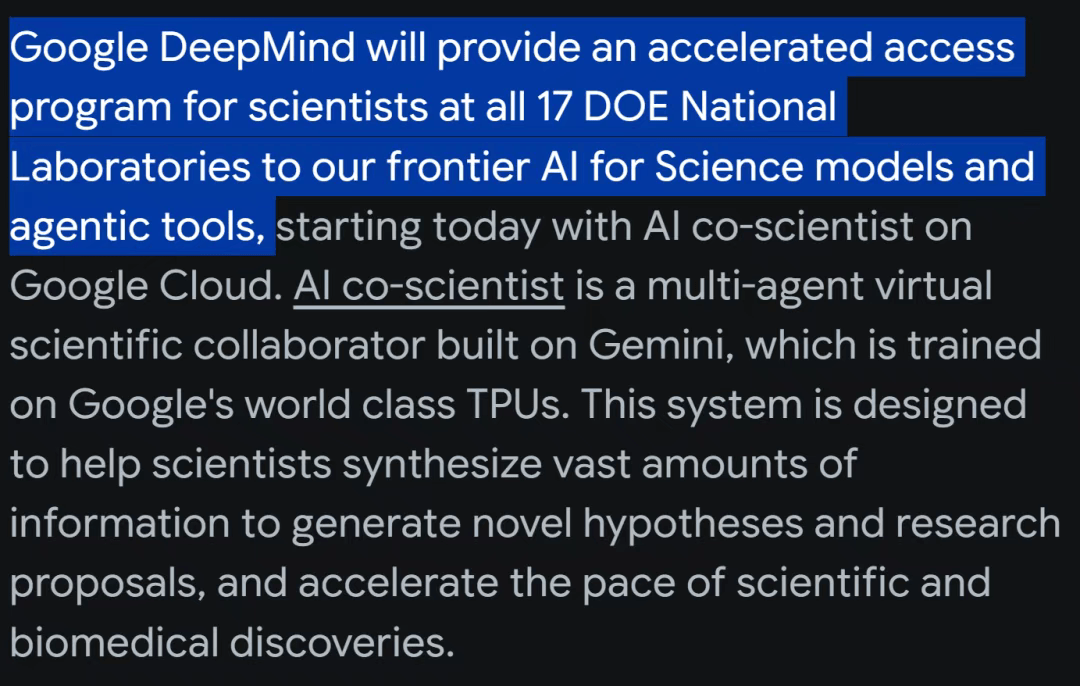
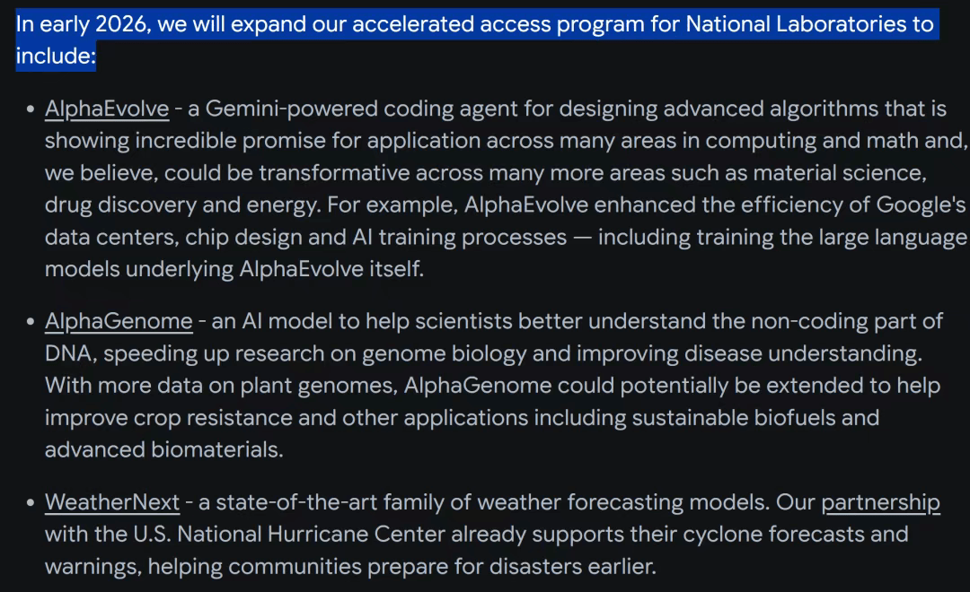
2025年的后半年,大家纷纷开始押注 AI for Science!
OpenAI 计划组建一个由顶尖学者组成的小型团队,这些学者需要满足三个条件:
这一系列举措表明,AI 驱动的科学发现正从学术探索迈向战略竞争新阶段。
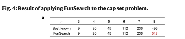
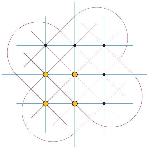
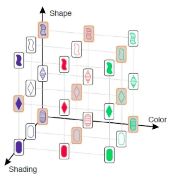
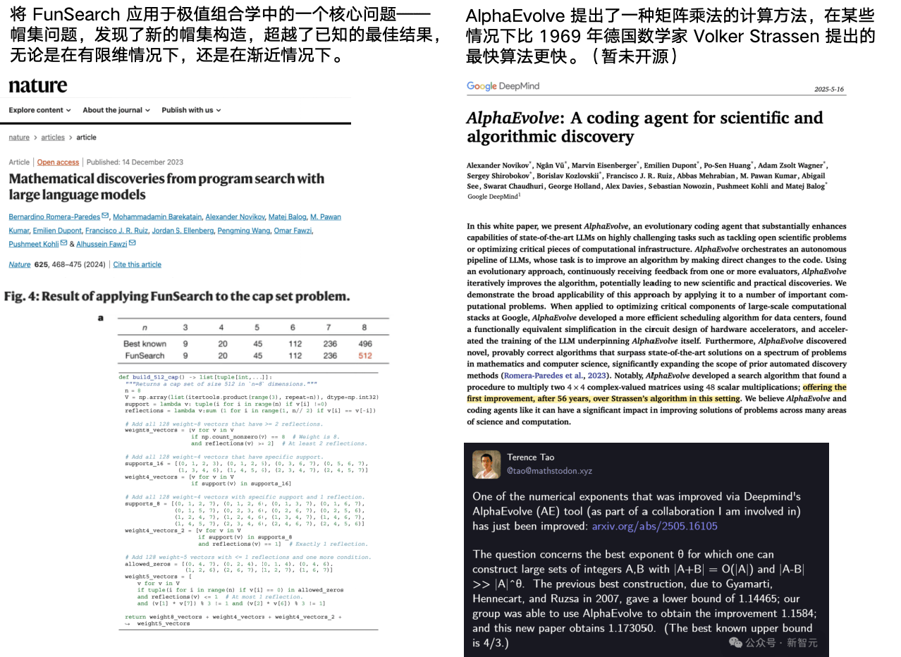
Cap Set Problem
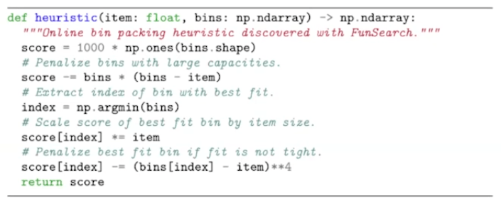
Bin Packing Problem
The largets cap set in N=2 has size 4.
The largest cap set in N=3 has size 9 > \(2^3\)
For N > 6, the size of the largest cap set is unknown.
Illustrative example of bin packing using existing heuristic – Best-fit heuristic (left), and using a heuristic discovered by FunSearch (right).
DeepMind Blog (Source)
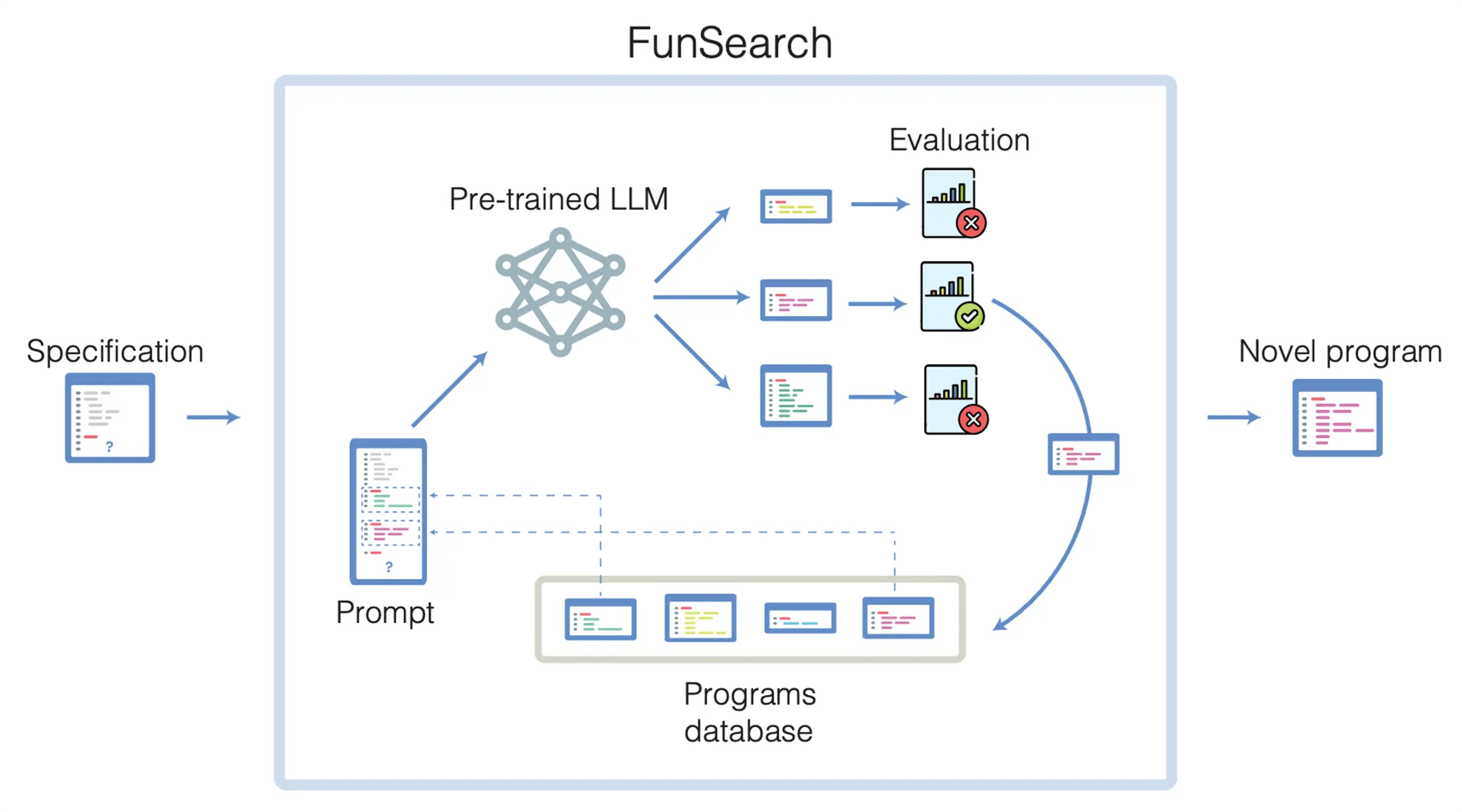
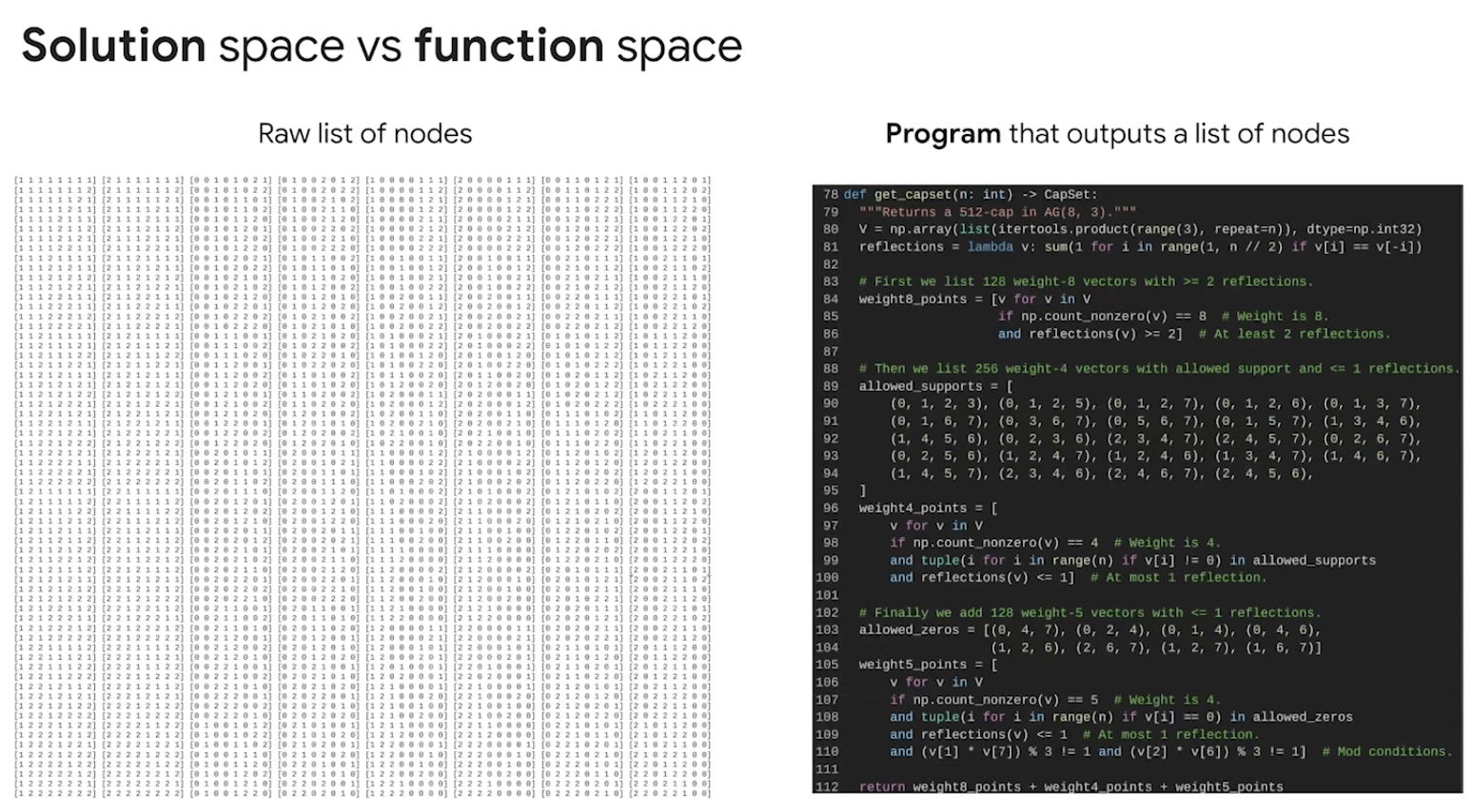
LLM guided search in ”program“ space
LLM guided search in ”program“ space
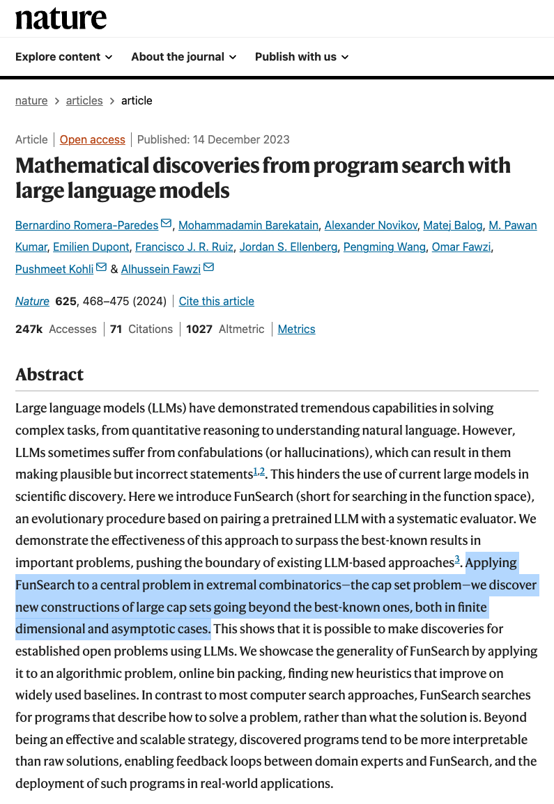
Real-world Case: FunSearch (Nature, 2023)
YouTube (Source)
YouTube (Source)
LLM guided search in ”program“ space
LLM guided search in ”program“ space
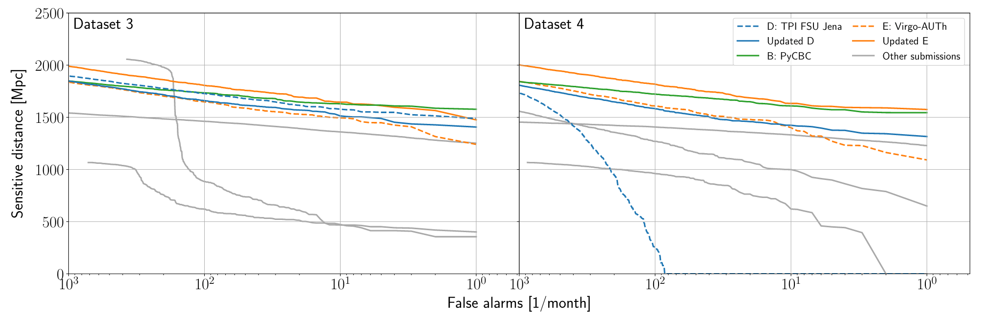
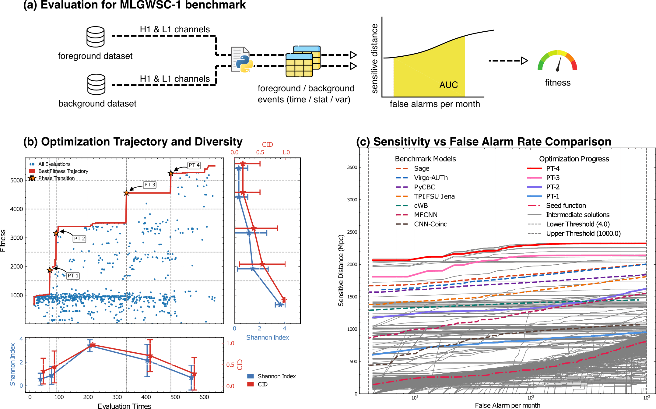
Evaluation for MLGWSC-1 benchmark
Concept
Mechanism
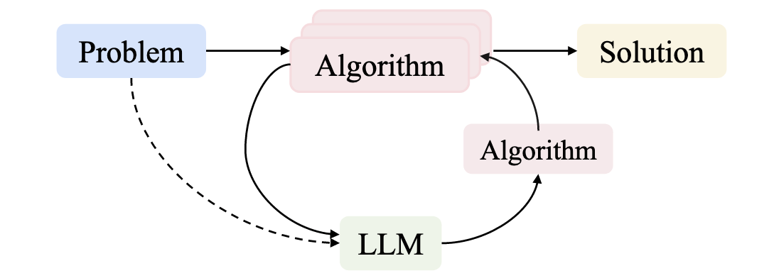
problem → algorithm
data → algorithm → reward
↺ LLM-guided algorithm updates
from problem-solving to algorithm discovery
HW, LZ. arXiv:2508.03661 [cs.AI]
The LLM does not predict answers — it reshapes how we search for algorithms.
LLMs act as policies over algorithms, not predictors of data.
external_knowledge
(constraint)
Evaluation for MLGWSC-1 benchmark
LLM as designer
arXiv:2410.14716 [cs.LG]
import numpy as np
import scipy.signal as signal
def pipeline_v1(strain_h1: np.ndarray, strain_l1: np.ndarray, times: np.ndarray) -> tuple[np.ndarray, np.ndarray, np.ndarray]:
    def data_conditioning(strain_h1: np.ndarray, strain_l1: np.ndarray, times: np.ndarray) -> tuple[np.ndarray, np.ndarray, np.ndarray]:
        window_length = 4096
        dt = times[1] - times[0]
        fs = 1.0 / dt

        def whiten_strain(strain):
            strain_zeromean = strain - np.mean(strain)
            freqs, psd = signal.welch(strain_zeromean, fs=fs, nperseg=window_length,
                                       window='hann', noverlap=window_length//2)
            smoothed_psd = np.convolve(psd, np.ones(32) / 32, mode='same')
            smoothed_psd = np.maximum(smoothed_psd, np.finfo(float).tiny)
            white_fft = np.fft.rfft(strain_zeromean) / np.sqrt(np.interp(np.fft.rfftfreq(len(strain_zeromean), d=dt), freqs, smoothed_psd))
            return np.fft.irfft(white_fft)

        whitened_h1 = whiten_strain(strain_h1)
        whitened_l1 = whiten_strain(strain_l1)

        return whitened_h1, whitened_l1, times

    def compute_metric_series(h1_data: np.ndarray, l1_data: np.ndarray, time_series: np.ndarray) -> tuple[np.ndarray, np.ndarray]:
        fs = 1 / (time_series[1] - time_series[0])
        f_h1, t_h1, Sxx_h1 = signal.spectrogram(h1_data, fs=fs, nperseg=256, noverlap=128, mode='magnitude', detrend=False)
        f_l1, t_l1, Sxx_l1 = signal.spectrogram(l1_data, fs=fs, nperseg=256, noverlap=128, mode='magnitude', detrend=False)
        tf_metric = np.mean((Sxx_h1**2 + Sxx_l1**2) / 2, axis=0)
        gps_mid_time = time_series[0] + (time_series[-1] - time_series[0]) / 2
        metric_times = gps_mid_time + (t_h1 - t_h1[-1] / 2)

        return tf_metric, metric_times

    def calculate_statistics(tf_metric, t_h1):
        background_level = np.median(tf_metric)
        peaks, _ = signal.find_peaks(tf_metric, height=background_level * 1.0, distance=2, prominence=background_level * 0.3)
        peak_times = t_h1[peaks]
        peak_heights = tf_metric[peaks]
        peak_deltat = np.full(len(peak_times), 10.0)  # Fixed uncertainty value
        return peak_times, peak_heights, peak_deltat

    whitened_h1, whitened_l1, data_times = data_conditioning(strain_h1, strain_l1, times)
    tf_metric, metric_times = compute_metric_series(whitened_h1, whitened_l1, data_times)
    peak_times, peak_heights, peak_deltat = calculate_statistics(tf_metric, metric_times)

    return peak_times, peak_heights, peak_deltat
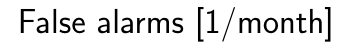
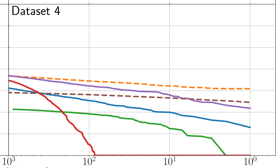
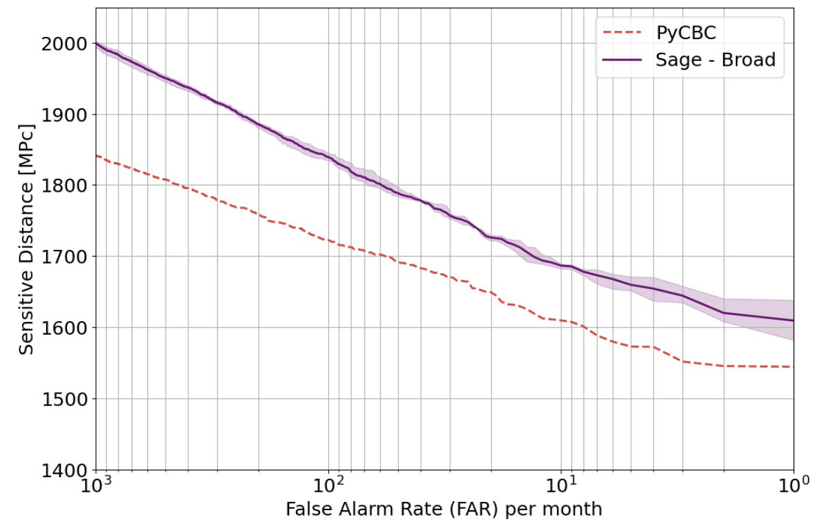
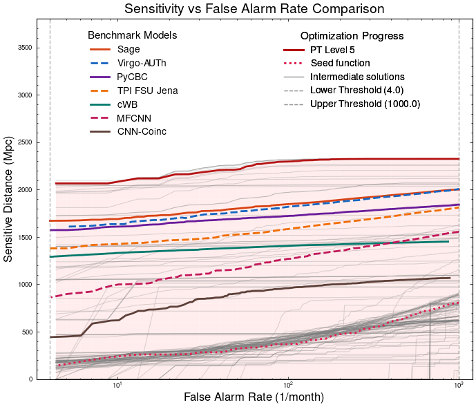
Optimization Target: Maximizing Area Under Curve (AUC) in the 1-1000Hz false alarms per-year range, balancing detection sensitivity and false alarm rates across algorithm generations
MLGWSC-1 benchmark
HW, LZ. arXiv:2508.03661 [cs.AI]
The LLM does not predict answers — it reshapes how we search for algorithms.
LLMs act as policies over algorithms, not predictors of data.
external_knowledge
(constraint)
PyCBC (linear-core)
cWB (nonlinear-core)
Simple filters (non-linear)
CNN-like (highly non-linear)
Benchmarking against state-of-the-art methods
Evaluation for MLGWSC-1 benchmark
LLM as designer
arXiv:2410.14716 [cs.LG]
import numpy as np
import scipy.signal as signal
def pipeline_v1(strain_h1: np.ndarray, strain_l1: np.ndarray, times: np.ndarray) -> tuple[np.ndarray, np.ndarray, np.ndarray]:
    def data_conditioning(strain_h1: np.ndarray, strain_l1: np.ndarray, times: np.ndarray) -> tuple[np.ndarray, np.ndarray, np.ndarray]:
        window_length = 4096
        dt = times[1] - times[0]
        fs = 1.0 / dt

        def whiten_strain(strain):
            strain_zeromean = strain - np.mean(strain)
            freqs, psd = signal.welch(strain_zeromean, fs=fs, nperseg=window_length,
                                       window='hann', noverlap=window_length//2)
            smoothed_psd = np.convolve(psd, np.ones(32) / 32, mode='same')
            smoothed_psd = np.maximum(smoothed_psd, np.finfo(float).tiny)
            white_fft = np.fft.rfft(strain_zeromean) / np.sqrt(np.interp(np.fft.rfftfreq(len(strain_zeromean), d=dt), freqs, smoothed_psd))
            return np.fft.irfft(white_fft)

        whitened_h1 = whiten_strain(strain_h1)
        whitened_l1 = whiten_strain(strain_l1)

        return whitened_h1, whitened_l1, times

    def compute_metric_series(h1_data: np.ndarray, l1_data: np.ndarray, time_series: np.ndarray) -> tuple[np.ndarray, np.ndarray]:
        fs = 1 / (time_series[1] - time_series[0])
        f_h1, t_h1, Sxx_h1 = signal.spectrogram(h1_data, fs=fs, nperseg=256, noverlap=128, mode='magnitude', detrend=False)
        f_l1, t_l1, Sxx_l1 = signal.spectrogram(l1_data, fs=fs, nperseg=256, noverlap=128, mode='magnitude', detrend=False)
        tf_metric = np.mean((Sxx_h1**2 + Sxx_l1**2) / 2, axis=0)
        gps_mid_time = time_series[0] + (time_series[-1] - time_series[0]) / 2
        metric_times = gps_mid_time + (t_h1 - t_h1[-1] / 2)

        return tf_metric, metric_times

    def calculate_statistics(tf_metric, t_h1):
        background_level = np.median(tf_metric)
        peaks, _ = signal.find_peaks(tf_metric, height=background_level * 1.0, distance=2, prominence=background_level * 0.3)
        peak_times = t_h1[peaks]
        peak_heights = tf_metric[peaks]
        peak_deltat = np.full(len(peak_times), 10.0)  # Fixed uncertainty value
        return peak_times, peak_heights, peak_deltat

    whitened_h1, whitened_l1, data_times = data_conditioning(strain_h1, strain_l1, times)
    tf_metric, metric_times = compute_metric_series(whitened_h1, whitened_l1, data_times)
    peak_times, peak_heights, peak_deltat = calculate_statistics(tf_metric, metric_times)

    return peak_times, peak_heights, peak_deltat
HW, LZ. arXiv:2508.03661 [cs.AI]
The LLM does not predict answers — it reshapes how we search for algorithms.
LLMs act as policies over algorithms, not predictors of data.
AI and Cosmology: From Computational Tools to Scientific Discovery
You are an expert in gravitational wave signal detection algorithms. Your task is to design heuristics that can effectively solve optimization problems.
{prompt_task}
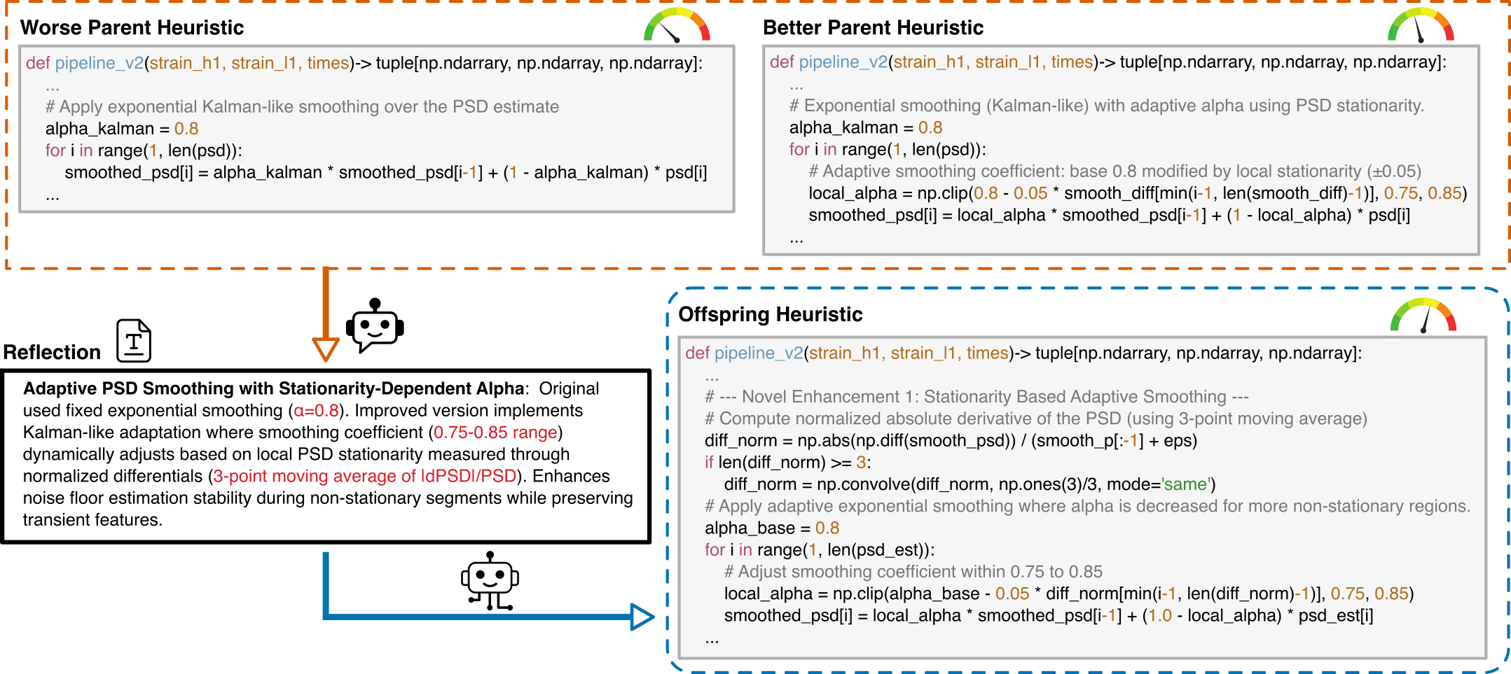
I have analyzed two algorithms and provided a reflection on their differences.
[Worse code]
{worse_code}
[Better code]
{better_code}
[Reflection]
{reflection}
{external_knowledge}
Based on this reflection, please write an improved algorithm according to the reflection.
First, describe the design idea and main steps of your algorithm in one sentence. The description must be inside a brace outside the code implementation. Next, implement it in Python as a function named '{func_name}'.
This function should accept {input_count} input(s): {joined_inputs}. The function should return {output_count} output(s): {joined_outputs}.
{inout_inf} {other_inf}
Do not give additional explanations.One Prompt Template for MLGWSC1 Algorithm Synthesis
LLM as designer
external_knowledge
(constraint)
arXiv:2410.14716 [cs.LG]
The LLM does not predict answers — it reshapes how we search for algorithms.
LLMs act as policies over algorithms, not predictors of data.
AI and Cosmology: From Computational Tools to Scientific Discovery
LLM as designer
external_knowledge
(constraint)
arXiv:2410.14716 [cs.LG]
The LLM does not predict answers — it reshapes how we search for algorithms.
LLMs act as policies over algorithms, not predictors of data.
AI and Cosmology: From Computational Tools to Scientific Discovery
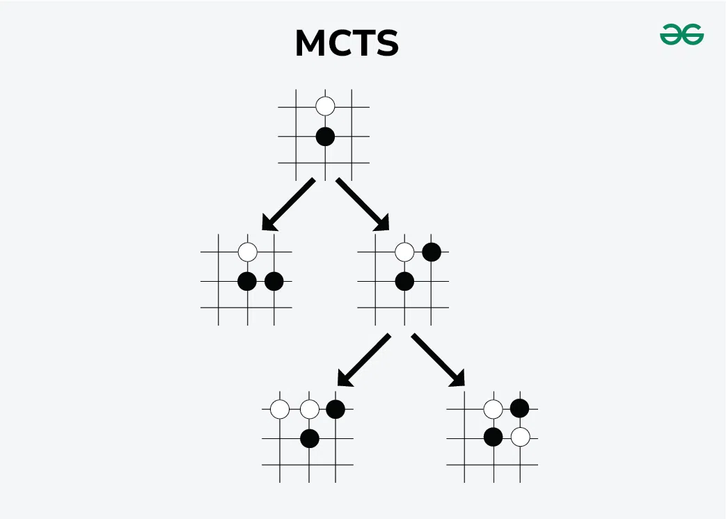
MCTS
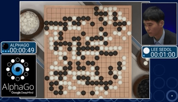
Casse1: Go Game
Case 2: OpenAI Strawberry (o1)
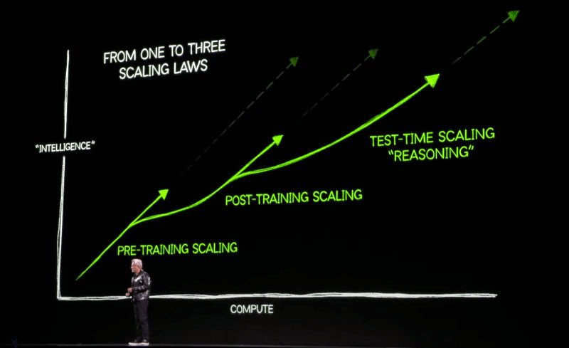
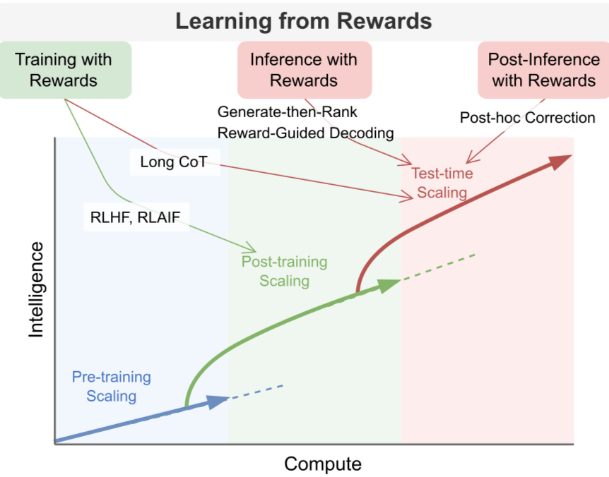
The release of o1 marks the formal deployment of the inference-time scaling paradigm in production. As Richard Sutton pointed out in The Bitter Lesson, only learning and search are methods that can scale indefinitely with compute. From this point on, the focus has increasingly shifted toward search.
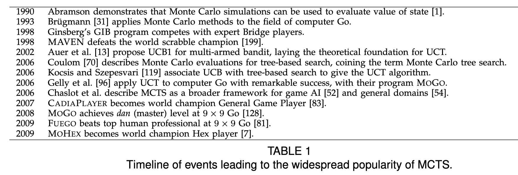
Browne et al. (2012)
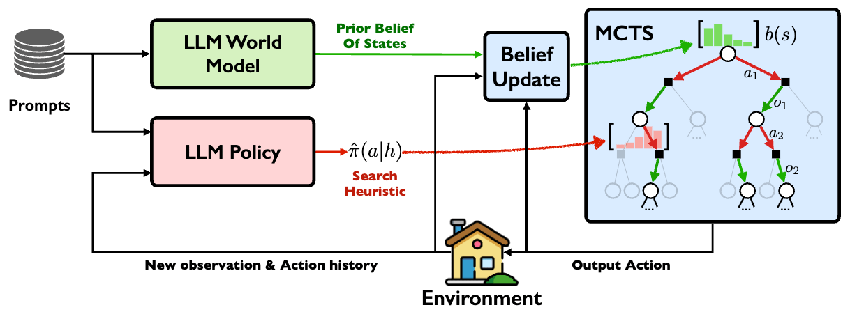
arXiv:2305.14078 [cs.RO]
Monte Carlo Tree Search (MCTS), which combines stochastic simulation with tree-based search to optimize decision-making, has long been a core technique in modern game-playing systems such as AlphaGo.
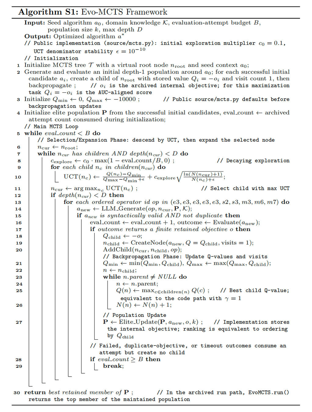
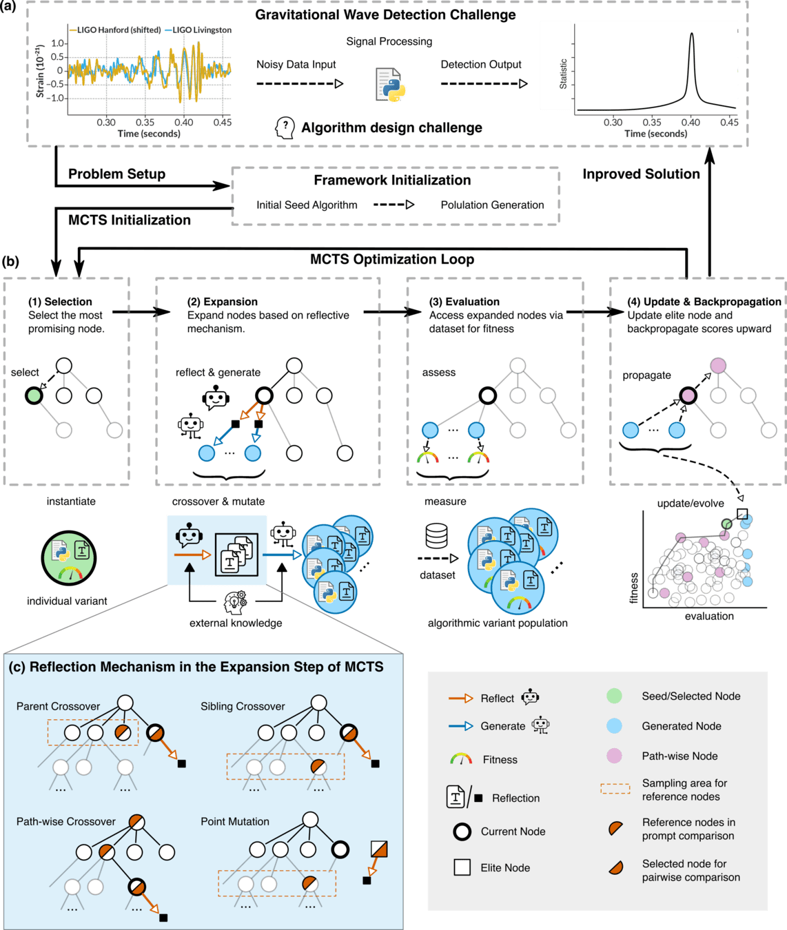
LLM-Informed Evo-MCTS
AI and Cosmology: From Computational Tools to Scientific Discovery
LLM-Informed Evo-MCTS
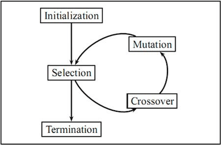
EA
Evolutionary Algorithms (EAs) are a class of heuristic search methods that simulate the mechanisms of biological evolution in nature, such as selection, crossover, and mutation. Their main advantages include:
LLM-Driven Algorithmic Evolution Through Reflective Code Synthesis.
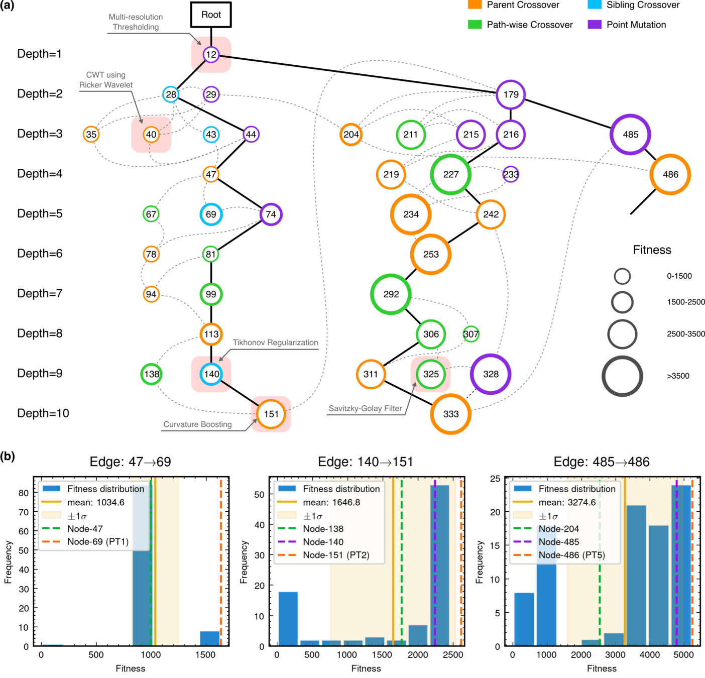
Monte Carlo Tree Search (MCTS) Algorithmic Evolution Pathway
What changed?
LLMs propose actions that guide the search
Evaluations (fitness/likelihood/...) become reusable memory
HW, LZ. arXiv:2508.03661 [cs.AI]
The LLM does not predict answers — it reshapes how we search for algorithms.
Search trajectories matter more than isolated optima.
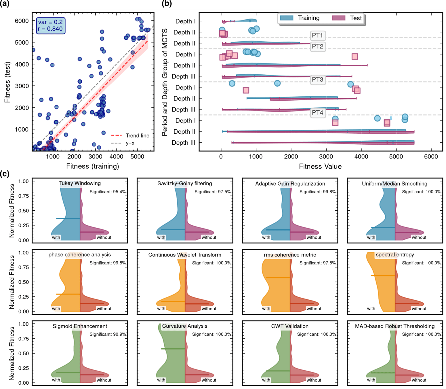
Algorithmic Component Impact Analysis.
import numpy as np
import scipy.signal as signal
from scipy.signal.windows import tukey
from scipy.signal import savgol_filter

def pipeline_v2(strain_h1: np.ndarray, strain_l1: np.ndarray, times: np.ndarray) -> tuple[np.ndarray, np.ndarray, np.ndarray]:
    """
    The pipeline function processes gravitational wave data from the H1 and L1 detectors to identify potential gravitational wave signals.
    It takes strain_h1 and strain_l1 numpy arrays containing detector data, and times array with corresponding time points.
    The function returns a tuple of three numpy arrays: peak_times containing GPS times of identified events,
    peak_heights with significance values of each peak, and peak_deltat showing time window uncertainty for each peak.
    """
    eps = np.finfo(float).tiny
    dt = times[1] - times[0]
    fs = 1.0 / dt
    # Base spectrogram parameters
    base_nperseg = 256
    base_noverlap = base_nperseg // 2
    medfilt_kernel = 101       # odd kernel size for robust detrending
    uncertainty_window = 5     # half-window for local timing uncertainty

    # -------------------- Stage 1: Robust Baseline Detrending --------------------
    # Remove long-term trends using a median filter for each channel.
    detrended_h1 = strain_h1 - signal.medfilt(strain_h1, kernel_size=medfilt_kernel)
    detrended_l1 = strain_l1 - signal.medfilt(strain_l1, kernel_size=medfilt_kernel)

    # -------------------- Stage 2: Adaptive Whitening with Enhanced PSD Smoothing --------------------
    def adaptive_whitening(strain: np.ndarray) -> np.ndarray:
        # Center the signal.
        centered = strain - np.mean(strain)
        n_samples = len(centered)
        # Adaptive window length: between 5 and 30 seconds
        win_length_sec = np.clip(n_samples / fs / 20, 5, 30)
        nperseg_adapt = int(win_length_sec * fs)
        nperseg_adapt = max(10, min(nperseg_adapt, n_samples))

        # Create a Tukey window with 75% overlap.
        tukey_alpha = 0.25
        win = tukey(nperseg_adapt, alpha=tukey_alpha)
        noverlap_adapt = int(nperseg_adapt * 0.75)
        if noverlap_adapt >= nperseg_adapt:
            noverlap_adapt = nperseg_adapt - 1

        # Estimate the power spectral density (PSD) using Welch's method.
        freqs, psd = signal.welch(centered, fs=fs, nperseg=nperseg_adapt,
                                  noverlap=noverlap_adapt, window=win, detrend='constant')
        psd = np.maximum(psd, eps)

        # Compute relative differences for PSD stationarity measure.
        diff_arr = np.abs(np.diff(psd)) / (psd[:-1] + eps)
        # Smooth the derivative with a moving average.
        if len(diff_arr) >= 3:
            smooth_diff = np.convolve(diff_arr, np.ones(3)/3, mode='same')
        else:
            smooth_diff = diff_arr

        # Exponential smoothing (Kalman-like) with adaptive alpha using PSD stationarity.
        smoothed_psd = np.copy(psd)
        for i in range(1, len(psd)):
            # Adaptive smoothing coefficient: base 0.8 modified by local stationarity (±0.05)
            local_alpha = np.clip(0.8 - 0.05 * smooth_diff[min(i-1, len(smooth_diff)-1)], 0.75, 0.85)
            smoothed_psd[i] = local_alpha * smoothed_psd[i-1] + (1 - local_alpha) * psd[i]

        # Compute Tikhonov regularization gain based on deviation from median PSD.
        noise_baseline = np.median(smoothed_psd)
        raw_gain = (smoothed_psd / (noise_baseline + eps)) - 1.0

        # Compute a causal-like gradient using the Savitzky-Golay filter.
        win_len = 11 if len(smoothed_psd) >= 11 else ((len(smoothed_psd)//2)*2+1)
        polyorder = 2 if win_len > 2 else 1
        delta_freq = np.mean(np.diff(freqs))
        grad_psd = savgol_filter(smoothed_psd, win_len, polyorder, deriv=1, delta=delta_freq, mode='interp')

        # Nonlinear scaling via sigmoid to enhance gradient differences.
        sigmoid = lambda x: 1.0 / (1.0 + np.exp(-x))
        scaling_factor = 1.0 + 2.0 * sigmoid(np.abs(grad_psd) / (np.median(smoothed_psd) + eps))

        # Compute adaptive gain factors with nonlinear scaling.
        gain = 1.0 - np.exp(-0.5 * scaling_factor * raw_gain)
        gain = np.clip(gain, -8.0, 8.0)

        # FFT-based whitening: interpolate gain and PSD onto FFT frequency bins.
        signal_fft = np.fft.rfft(centered)
        freq_bins = np.fft.rfftfreq(n_samples, d=dt)
        interp_gain = np.interp(freq_bins, freqs, gain, left=gain[0], right=gain[-1])
        interp_psd = np.interp(freq_bins, freqs, smoothed_psd, left=smoothed_psd[0], right=smoothed_psd[-1])
        denom = np.sqrt(interp_psd) * (np.abs(interp_gain) + eps)
        denom = np.maximum(denom, eps)
        white_fft = signal_fft / denom
        whitened = np.fft.irfft(white_fft, n=n_samples)
        return whitened

    # Whiten H1 and L1 channels using the adapted method.
    white_h1 = adaptive_whitening(detrended_h1)
    white_l1 = adaptive_whitening(detrended_l1)

    # -------------------- Stage 3: Coherent Time-Frequency Metric with Frequency-Conditioned Regularization --------------------
    def compute_coherent_metric(w1: np.ndarray, w2: np.ndarray) -> tuple[np.ndarray, np.ndarray]:
        # Compute complex spectrograms preserving phase information.
        f1, t_spec, Sxx1 = signal.spectrogram(w1, fs=fs, nperseg=base_nperseg,
                                              noverlap=base_noverlap, mode='complex', detrend=False)
        f2, t_spec2, Sxx2 = signal.spectrogram(w2, fs=fs, nperseg=base_nperseg,
                                               noverlap=base_noverlap, mode='complex', detrend=False)
        # Ensure common time axis length.
        common_len = min(len(t_spec), len(t_spec2))
        t_spec = t_spec[:common_len]
        Sxx1 = Sxx1[:, :common_len]
        Sxx2 = Sxx2[:, :common_len]

        # Compute phase differences and coherence between detectors.
        phase_diff = np.angle(Sxx1) - np.angle(Sxx2)
        phase_coherence = np.abs(np.cos(phase_diff))

        # Estimate median PSD per frequency bin from the spectrograms.
        psd1 = np.median(np.abs(Sxx1)**2, axis=1)
        psd2 = np.median(np.abs(Sxx2)**2, axis=1)

        # Frequency-conditioned regularization gain (reflection-guided).
        lambda_f = 0.5 * ((np.median(psd1) / (psd1 + eps)) + (np.median(psd2) / (psd2 + eps)))
        lambda_f = np.clip(lambda_f, 1e-4, 1e-2)
        # Regularization denominator integrating detector PSDs and lambda.
        reg_denom = (psd1[:, None] + psd2[:, None] + lambda_f[:, None] + eps)

        # Weighted phase coherence that balances phase alignment with noise levels.
        weighted_comp = phase_coherence / reg_denom

        # Compute axial (frequency) second derivatives as curvature estimates.
        d2_coh = np.gradient(np.gradient(phase_coherence, axis=0), axis=0)
        avg_curvature = np.mean(np.abs(d2_coh), axis=0)

        # Nonlinear activation boost using tanh for regions of high curvature.
        nonlinear_boost = np.tanh(5 * avg_curvature)
        linear_boost = 1.0 + 0.1 * avg_curvature

        # Cross-detector synergy: weight derived from global median consistency.
        novel_weight = np.mean((np.median(psd1) + np.median(psd2)) / (psd1[:, None] + psd2[:, None] + eps), axis=0)

        # Integrated time-frequency metric combining all enhancements.
        tf_metric = np.sum(weighted_comp * linear_boost * (1.0 + nonlinear_boost), axis=0) * novel_weight

        # Adjust the spectrogram time axis to account for window delay.
        metric_times = t_spec + times[0] + (base_nperseg / 2) / fs
        return tf_metric, metric_times

    tf_metric, metric_times = compute_coherent_metric(white_h1, white_l1)

    # -------------------- Stage 4: Multi-Resolution Thresholding with Octave-Spaced Dyadic Wavelet Validation --------------------
    def multi_resolution_thresholding(metric: np.ndarray, times_arr: np.ndarray) -> tuple[np.ndarray, np.ndarray, np.ndarray]:
        # Robust background estimation with median and MAD.
        bg_level = np.median(metric)
        mad_val = np.median(np.abs(metric - bg_level))
        robust_std = 1.4826 * mad_val
        threshold = bg_level + 1.5 * robust_std

        # Identify candidate peaks using prominence and minimum distance criteria.
        peaks, _ = signal.find_peaks(metric, height=threshold, distance=2, prominence=0.8 * robust_std)
        if peaks.size == 0:
            return np.array([]), np.array([]), np.array([])

        # Local uncertainty estimation using a Gaussian-weighted convolution.
        win_range = np.arange(-uncertainty_window, uncertainty_window + 1)
        sigma = uncertainty_window / 2.5
        gauss_kernel = np.exp(-0.5 * (win_range / sigma) ** 2)
        gauss_kernel /= np.sum(gauss_kernel)
        weighted_mean = np.convolve(metric, gauss_kernel, mode='same')
        weighted_sq = np.convolve(metric ** 2, gauss_kernel, mode='same')
        variances = np.maximum(weighted_sq - weighted_mean ** 2, 0.0)
        uncertainties = np.sqrt(variances)
        uncertainties = np.maximum(uncertainties, 0.01)

        valid_times = []
        valid_heights = []
        valid_uncerts = []
        n_metric = len(metric)

        # Compute a simple second derivative for local curvature checking.
        if n_metric > 2:
            second_deriv = np.diff(metric, n=2)
            second_deriv = np.pad(second_deriv, (1, 1), mode='edge')
        else:
            second_deriv = np.zeros_like(metric)

        # Use octave-spaced scales (dyadic wavelet validation) to validate peak significance.
        widths = np.arange(1, 9)  # approximate scales 1 to 8
        for peak in peaks:
            # Skip peaks lacking sufficient negative curvature.
            if second_deriv[peak] > -0.1 * robust_std:
                continue
            local_start = max(0, peak - uncertainty_window)
            local_end = min(n_metric, peak + uncertainty_window + 1)
            local_segment = metric[local_start:local_end]
            if len(local_segment) < 3:
                continue
            try:
                cwt_coeff = signal.cwt(local_segment, signal.ricker, widths)
            except Exception:
                continue
            max_coeff = np.max(np.abs(cwt_coeff))
            # Threshold for validating the candidate using local MAD.
            cwt_thresh = mad_val * np.sqrt(2 * np.log(len(local_segment) + eps))
            if max_coeff >= cwt_thresh:
                valid_times.append(times_arr[peak])
                valid_heights.append(metric[peak])
                valid_uncerts.append(uncertainties[peak])

        if len(valid_times) == 0:
            return np.array([]), np.array([]), np.array([])
        return np.array(valid_times), np.array(valid_heights), np.array(valid_uncerts)

    peak_times, peak_heights, peak_deltat = multi_resolution_thresholding(tf_metric, metric_times)
return peak_times, peak_heights, peak_deltatPT Level 5
HW, LZ. arXiv:2508.03661 [cs.AI]
Integrated Architecture Validation
Contributions of knowledge synthesis
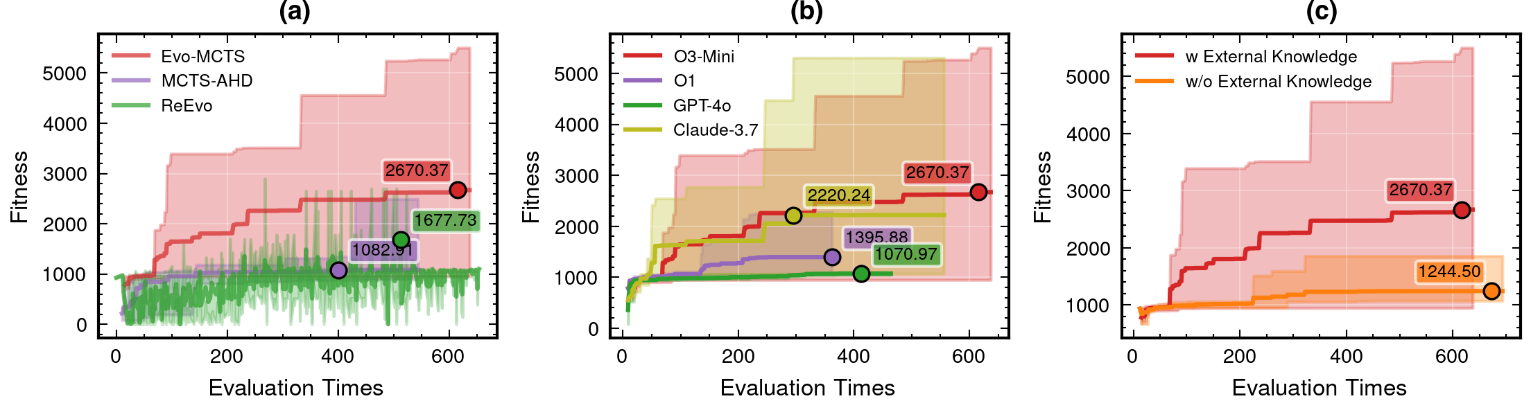
LLM Model Selection and Robustness Analysis
o3-mini-medium
o1-2024-12-17
gpt-4o-2024-11-20
claude-3-7-sonnet-20250219-thinking
59.1%
115%
HW, LZ. arXiv:2508.03661 [cs.AI]
AI and Cosmology: From Computational Tools to Scientific Discovery
Contributions of knowledge synthesis
59.1%
115%
59.1%
### External Knowledge Integration
1. **Non-linear** Processing Core Concepts:
    - Signal Transformation:
        * Non-linear vs linear decomposition
        * Adaptive threshold mechanisms
        * Multi-scale analysis

    - Feature Extraction:
        * Phase space reconstruction
        * Topological data analysis
        * Wavelet-based detection

    - Statistical Analysis:
        * Robust estimators
        * Non-Gaussian processes
        * Higher-order statistics

2. Implementation Principles:
    - Prioritize adaptive over fixed parameters
    - Consider local vs global characteristics
- Balance computational cost with accuracyHW, LZ. arXiv:2508.03661 [cs.AI]
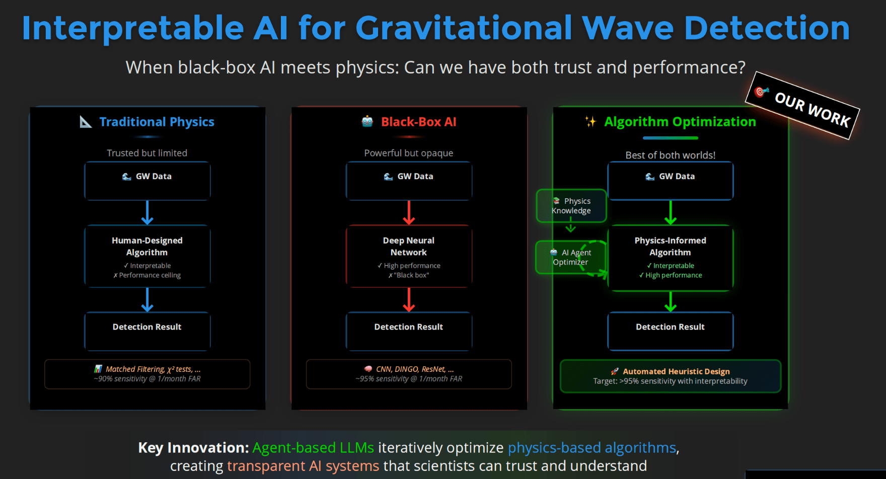
Interpretable AI Approach
The best of both worlds
Input
Physics-Informed
Algorithm
(High interpretability)
Output
Example: Evo-MCTS, AlphaEvolve
AI Model
Physics
Knowledge
Traditional Physics Approach
Input
Human-Designed Algorithm
(Based on human insight)
Output
Example: Matched Filtering, linear regression
Black-Box AI Approach
Input
AI Model
(Low interpretability)
Output
Examples: CNN, AlphaGo, DINGO
Data/
Experience
Data/
Experience
🎯 OUR WORK
Scientific discovery requires interpretability, not just performance.
Scientific discovery requires interpretability — not just performance.
vs
The design of any algorithm can be viewed as an optimization problem.
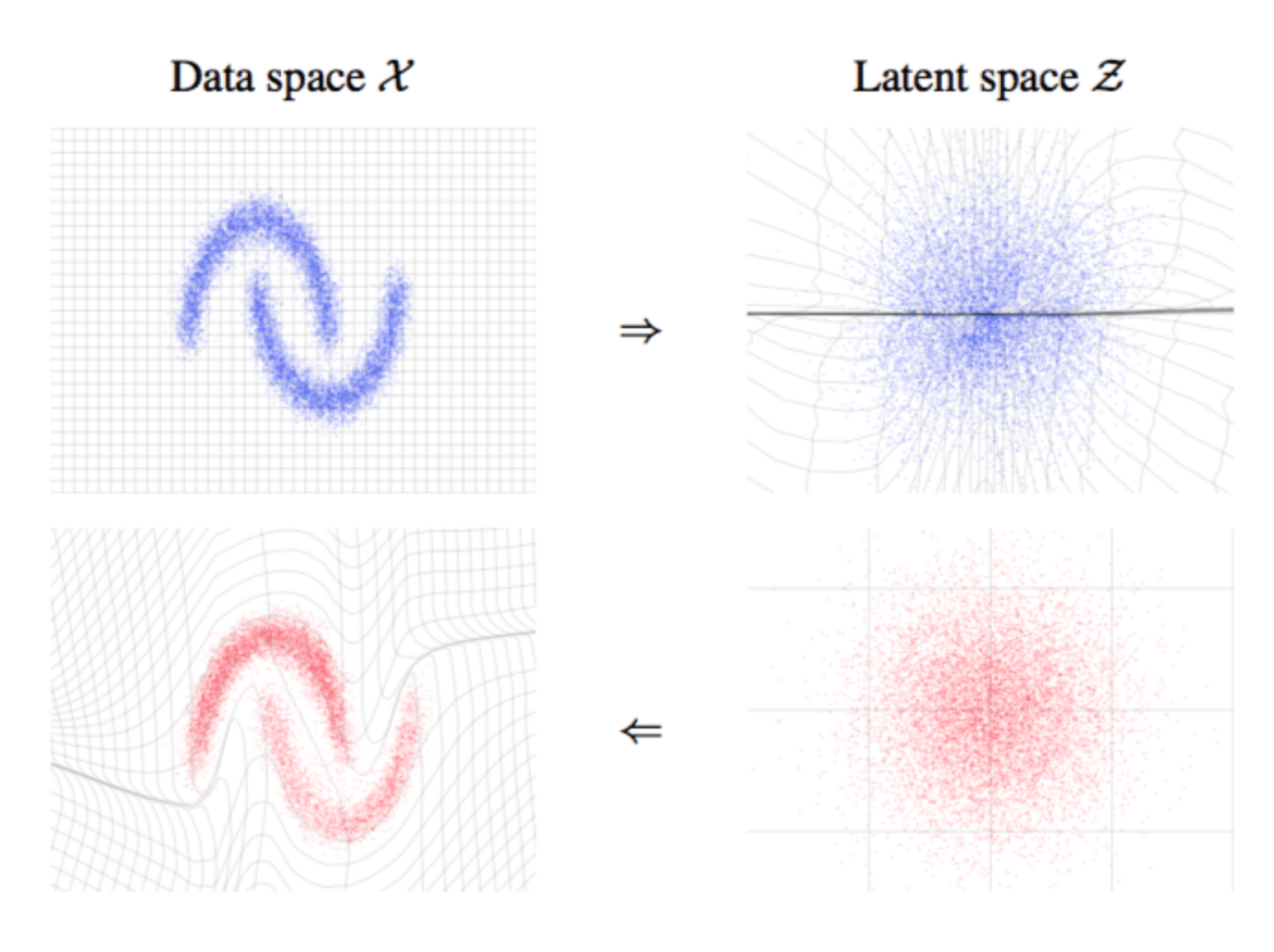
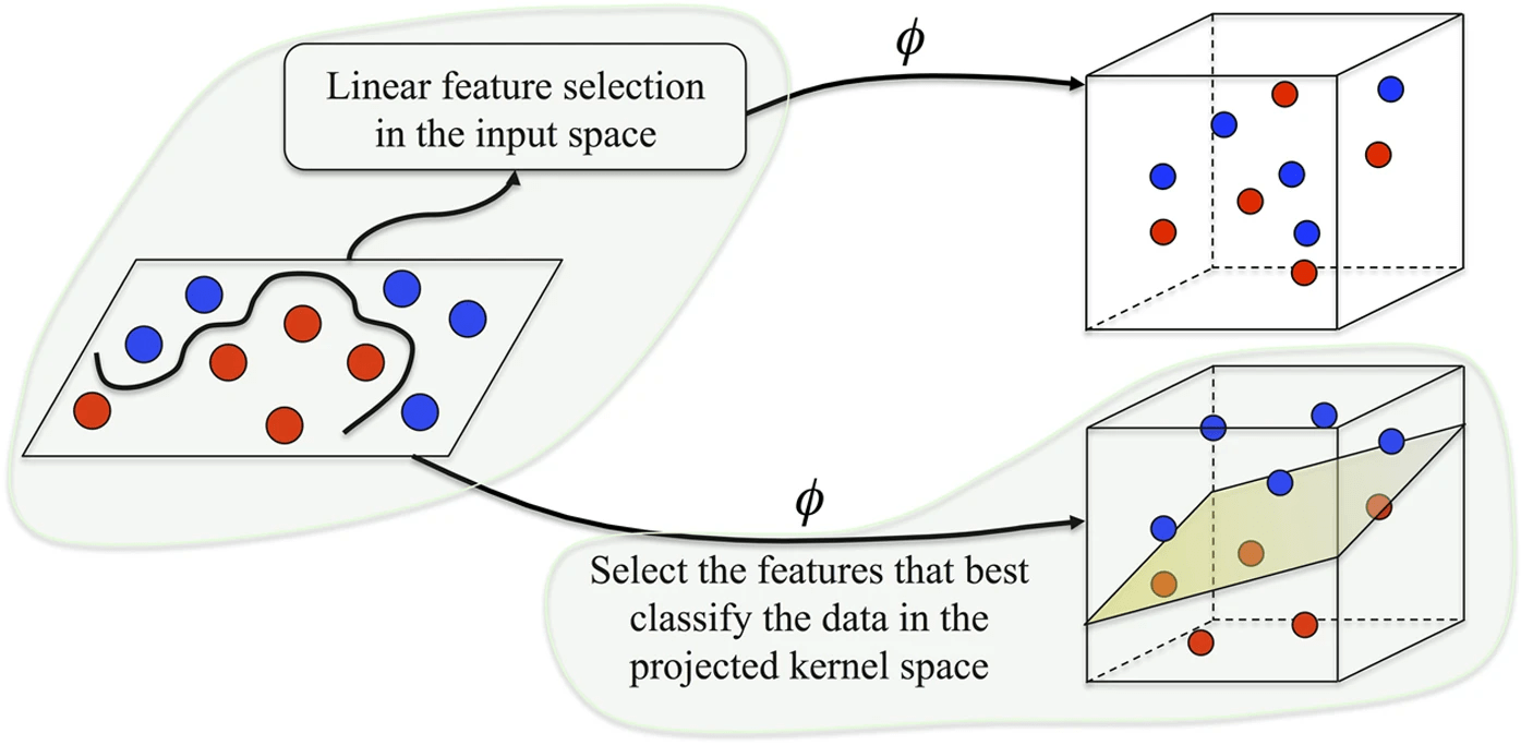
维度重构:从“信号匹配”到“特征提取” (Feature Extraction)
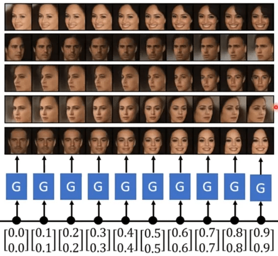
连续推断:从“离散采样”到“隐空间建模” (Latent Space Interpolation)
智能涌现:从“实验工具”到“科研合作者” (Nature of AI for Science)
for _ in range(num_of_audiences):
    print('Thank you for your attention! 🙏')
太极实验室 2026 年度“大学生创新实践训练计划’
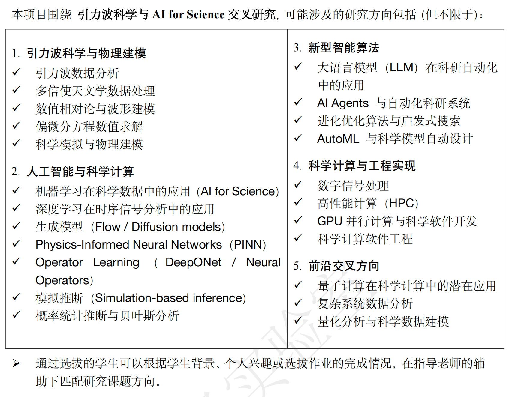
(引力波数据分析与 AI for Science 方向)
中国科学院大学引力波宇宙太极实验室(北京)引力波数据分析与机器学习课题组长期面向全国高校学生开放科研训练机会,现面向全国优秀学生招募参加太极实验室2026年度“大学生创新实践训练计划”,本课题组致力于探索引力波天文学、数值模拟与人工智能技术的交叉研究,重点发展新一代 Al for Science 方法,用于解决复杂物理系统建模、信号处理与科学数据分析问题,欢迎对 引力波科学、人工智能算法与科学计算 充满兴趣的同学加入,在真实科研项目中接受系统训练,并参与国际前沿研究。
https://github.com/iphysresearch/UndergradResearchLab/blob/main/2026科创计划及选拔题目.pdf
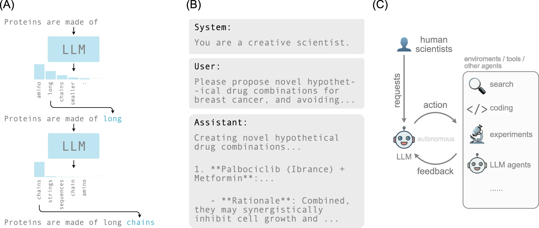
Uncovering the "black box" to reveal how LLM actually works
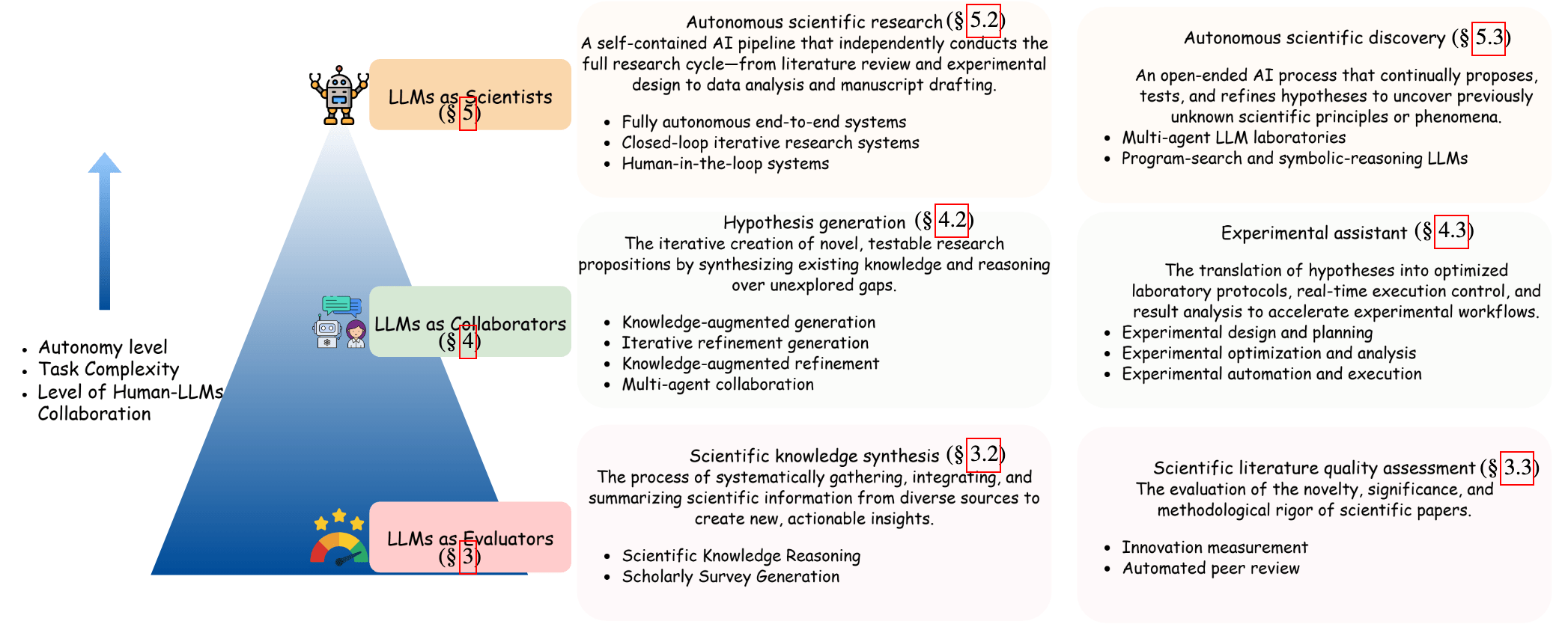
arXiv:2507.11810 [cs.DL]
"科学家"
"合作者"
"评估者"
Let's be honest about our motivations... 😉
AI and Cosmology: From Computational Tools to Scientific Discovery
Let's be honest about our motivations... 😉
直接不行?那就包装回炉再来一遍。
npj Artif. Intell. 1, 14 (2025).
"序列输出"
"序列输入"
Direct fails. Refine and recover.
AI and Cosmology: From Computational Tools to Scientific Discovery
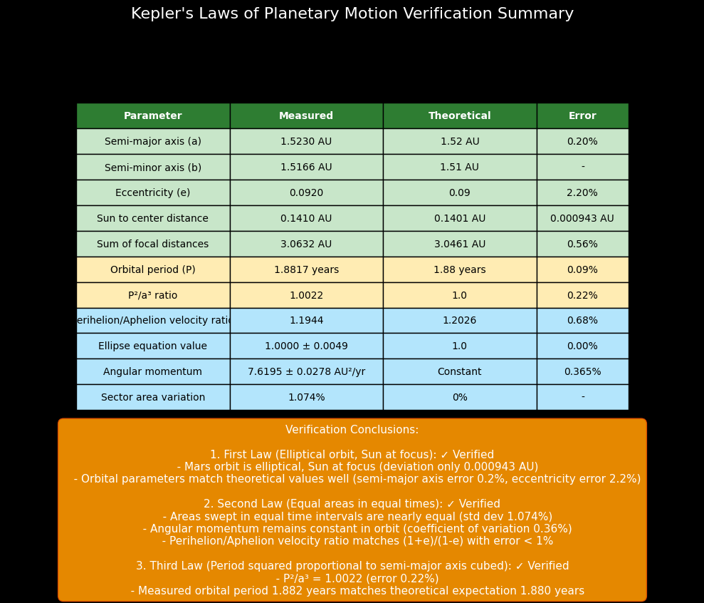
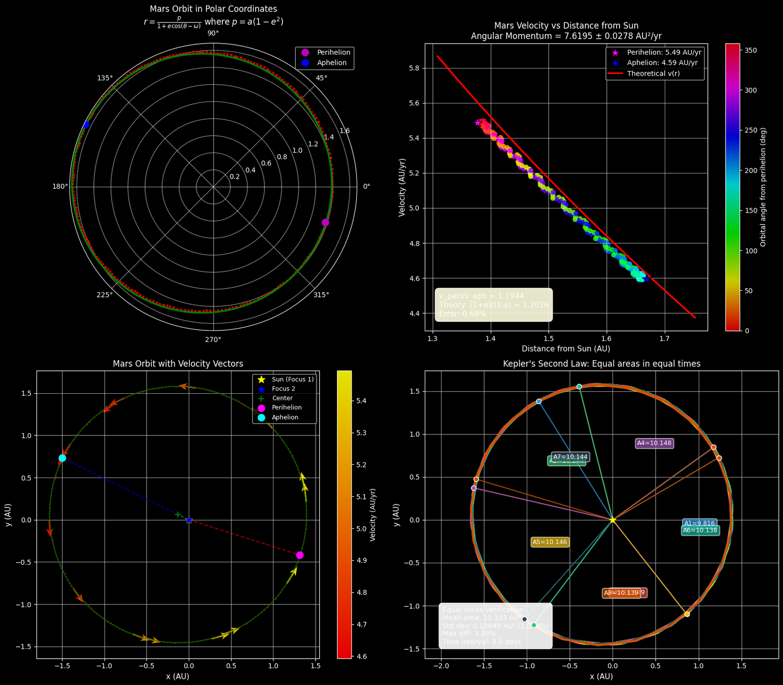
Demo: LLM 验证开普勒行星运动三定律 (2025.3)
Let's be honest about our motivations... 😉
AI and Cosmology: From Computational Tools to Scientific Discovery
Generative agents rely on predefined rules. 🤫
arXiv:2304.03442 [cs.HC]
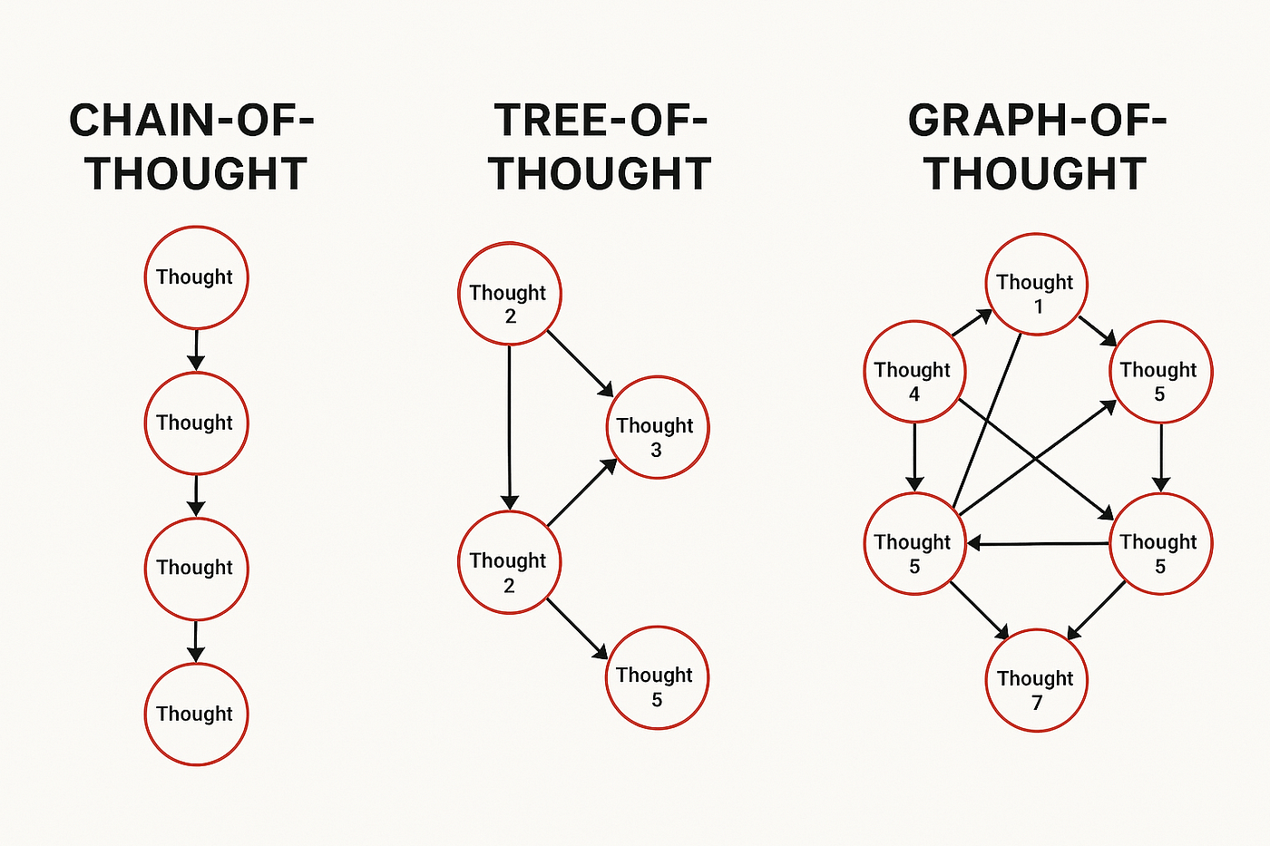
arXiv:2201.11903 [cs.CL]
arXiv:2305.10601 [cs.CL]
📄 Google DeepMind: "Scaling LLM Test-Time Compute Optimally" (arXiv:2408.03314)
🔗 OpenAI: Learning to Reason with LLMs
AI and Cosmology: From Computational Tools to Scientific Discovery
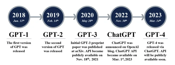
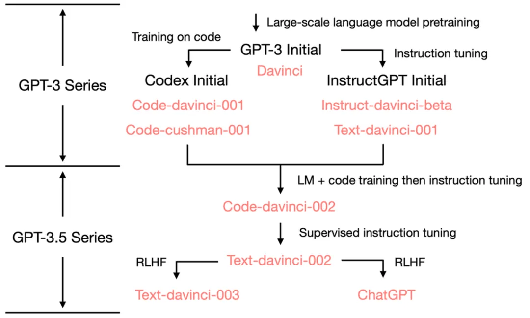
GPT能力的演变
对GPT-3.5能力的仔细审查揭示了其新兴能力的起源:
What are our thoughts on LLMs?
GPT-3.5 series [Source: University of Edinburgh, Allen Institute for AI]
GPT-3 (2020)
ChatGPT (2022)
Magic: Code + Text
究竟是什么让 LLMs 如此强大?
Code! (1/3)
AI and Cosmology: From Computational Tools to Scientific Discovery
What are our thoughts on LLMs?
究竟是什么让 LLMs 如此颠覆?
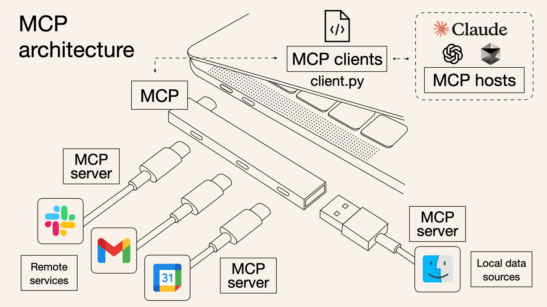
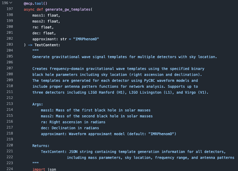
MCP
MCP Tool
prompt
"Please generate gw templates first."模型上下文协议(Model Context Protocol,MCP),是由Anthropic推出的开源协议,旨在实现大语言模型与外部数据源和工具的集成,用来在大模型和数据源之间建立安全双向的连接。
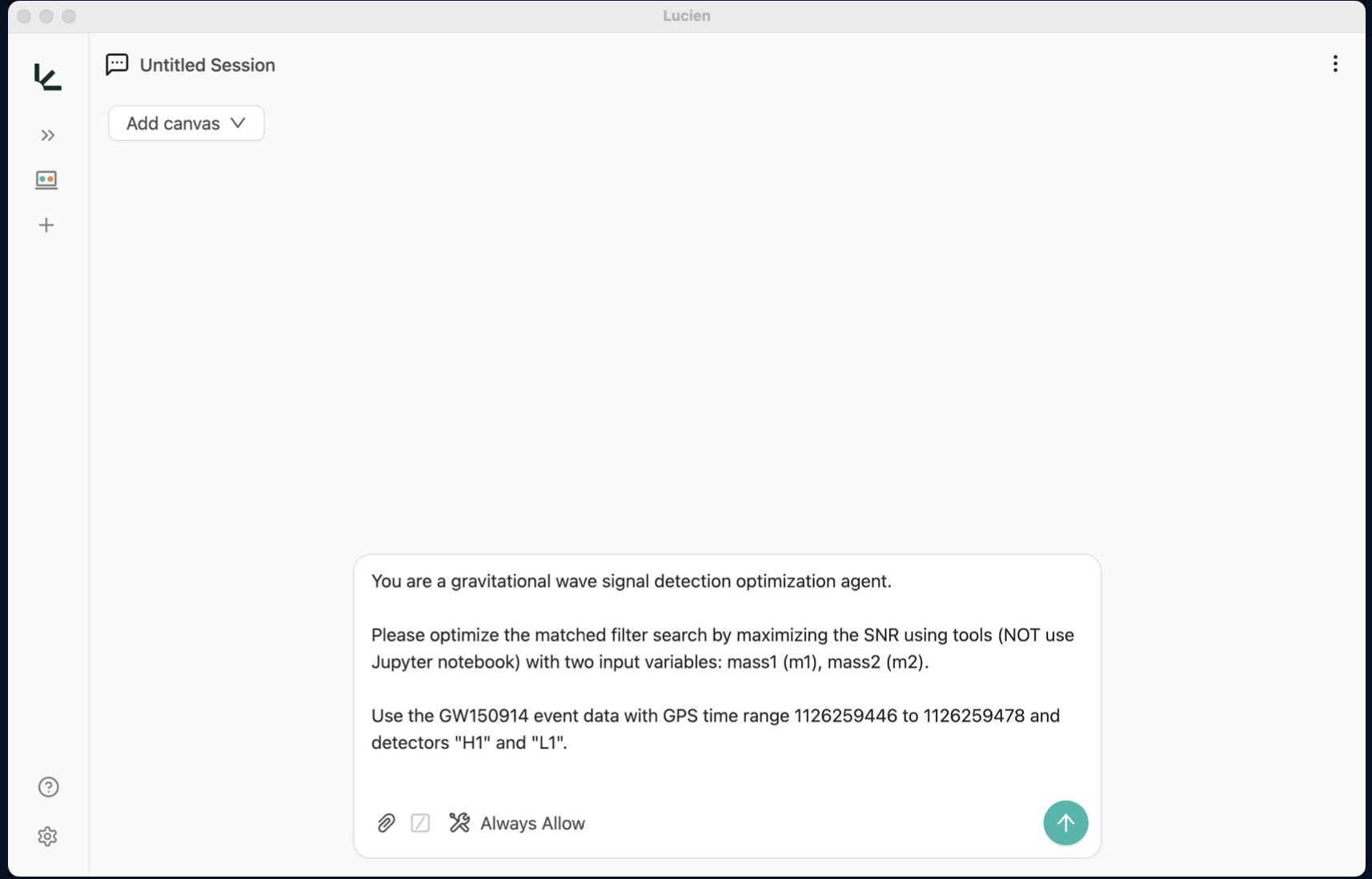
Demo: GW150914 MCP Signal Search
AI and Cosmology: From Computational Tools to Scientific Discovery
What are our thoughts on LLMs?
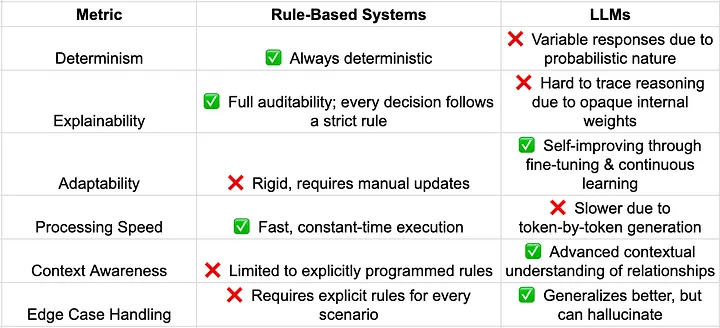
Rule-Based Vs. LLMs: (Source)
Natural Language Programming! (2/3)
究竟是什么让 LLMs 如此颠覆?
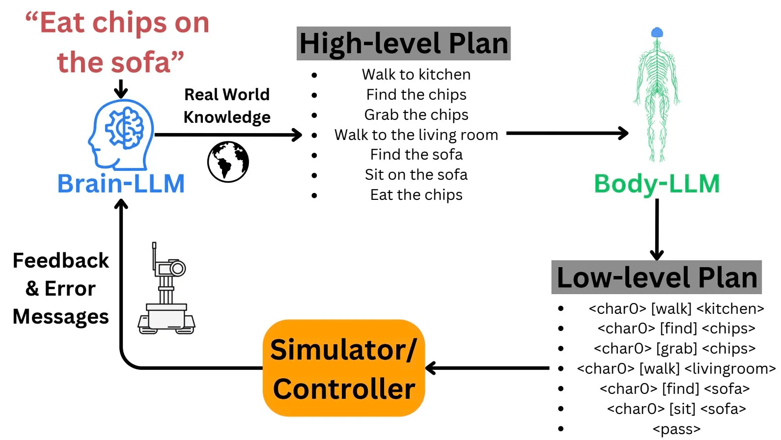
MCP
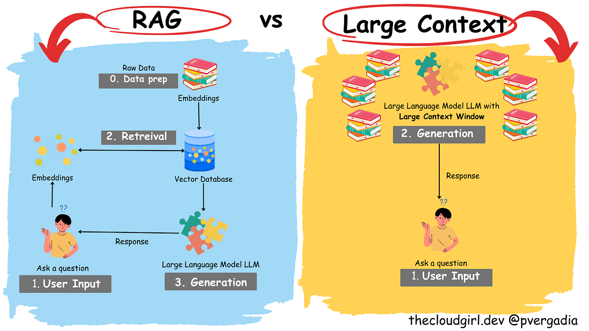
RAG
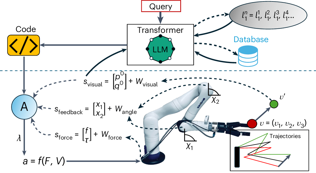
具身智能
AI and Cosmology: From Computational Tools to Scientific Discovery
What are our thoughts on LLMs?
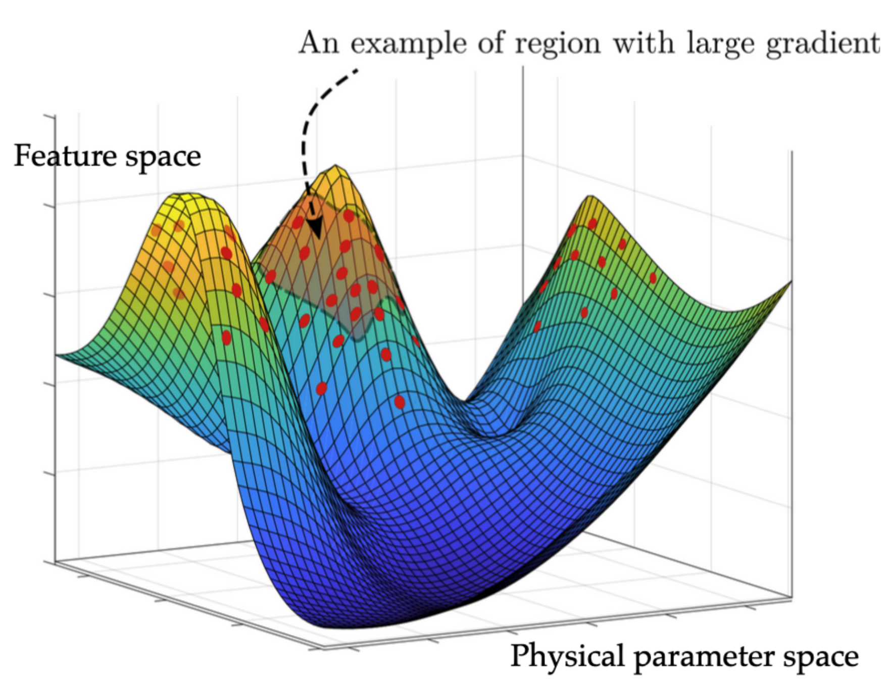
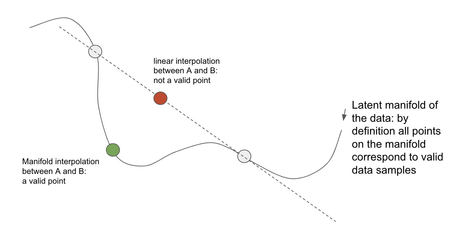
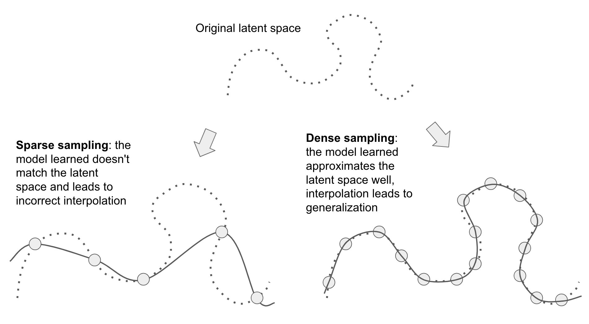
It's Mere Interpolation! (3/3)
究竟如何解释 AI/LLMs 的原理?
The core driving force of AI4Sci largely lies in its “interpolation” generalization capabilities, showcasing its powerful complex modeling abilities.
Deep Learning is Not As Impressive As you Think, It's Mere Interpolation (Source)
AI and Cosmology: From Computational Tools to Scientific Discovery
What are our thoughts on LLMs?
It's Mere Interpolation! (3/3)
究竟如何解释 AI/LLMs 的原理?
The core driving force of AI4Sci largely lies in its “interpolation” generalization capabilities, showcasing its powerful complex modeling abilities.
Deep Learning is Not As Impressive As you Think, It's Mere Interpolation (Source)
Representation Space Interpolation
Representation Space Interpolation
AI and Cosmology: From Computational Tools to Scientific Discovery
What are our thoughts on LLMs?
It's Mere Interpolation! (3/3)
究竟如何解释 AI/LLMs 的原理?
Deep Learning is Not As Impressive As you Think, It's Mere Interpolation (Source)
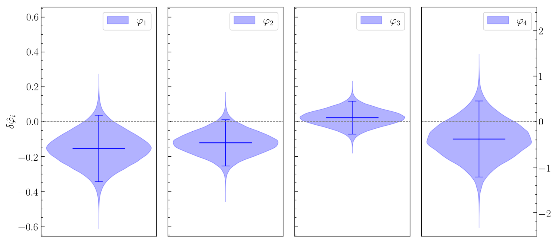
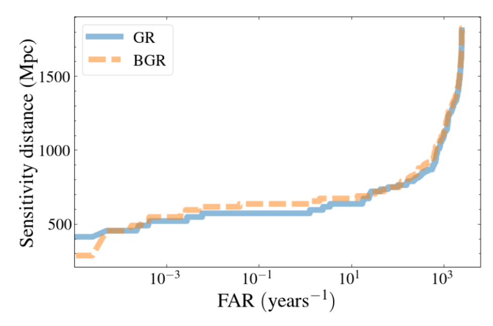
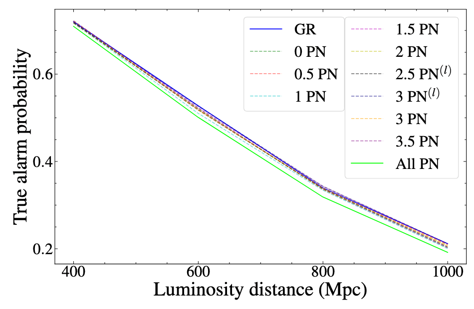
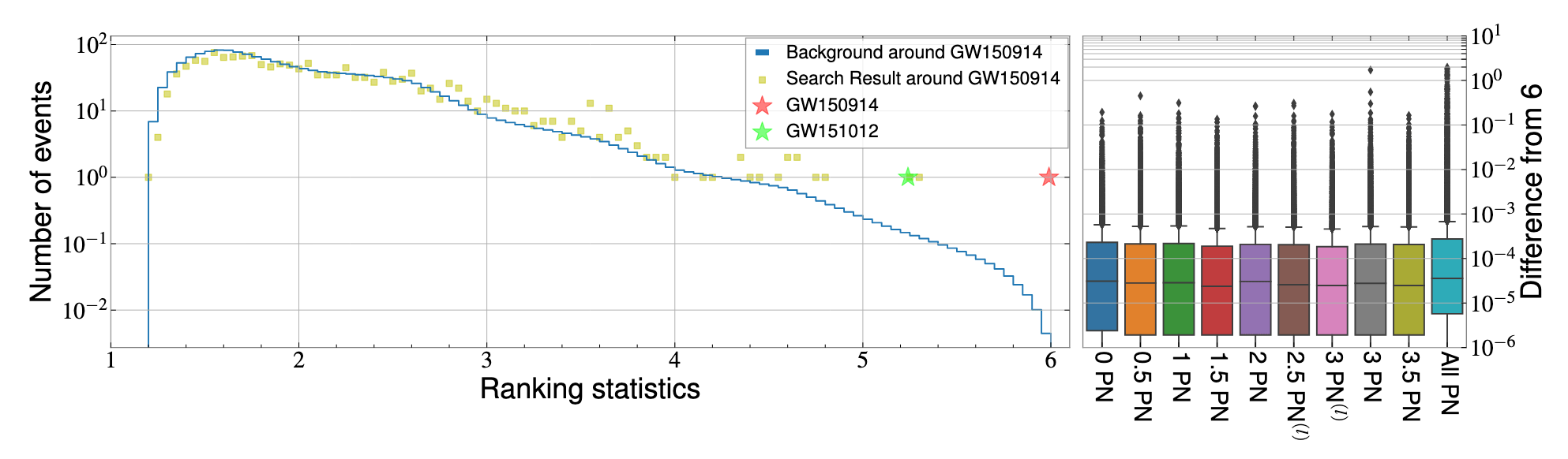
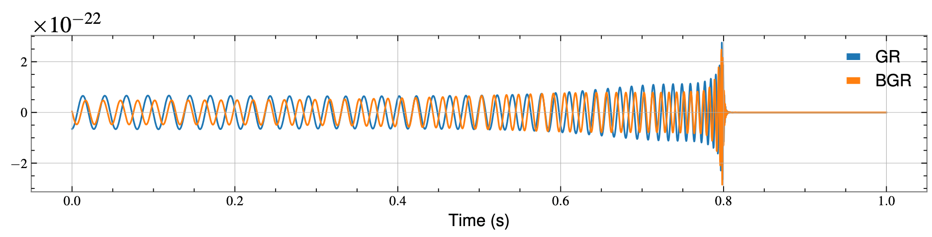
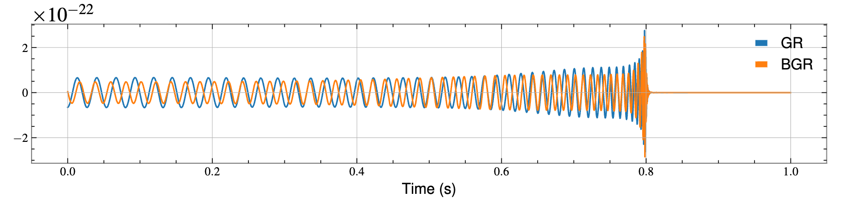
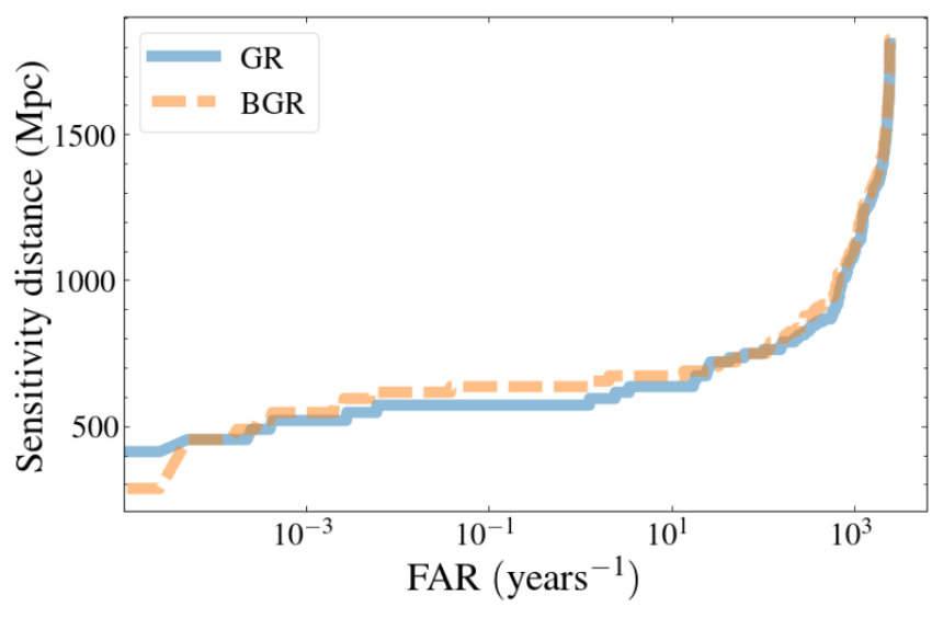
GR
BGR
Yu-Xin Wang, Xiaotong Wei, Chun-Yue Li, Tian-Yang Sun, Shang-Jie Jin, He Wang*, Jing-Lei Cui, Jing-Fei Zhang, and Xin Zhang*. “Search for Exotic Gravitational Wave Signals beyond General Relativity Using Deep Learning.” PRD 112 (2), 024030. e-Print: arXiv:2410.20129 [gr-qc]
~ sampling
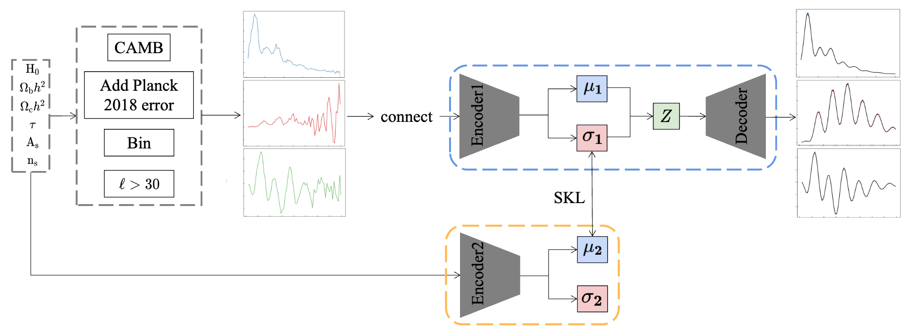
Tian-Yang Sun, Tian-Nuo Li, He Wang*, Jing-Fei Zhang, Xin Zhang*. Conditional variational autoencoders for cosmological model discrimination and anomaly detection in cosmic microwave background power spectra. e-Print: arxiv:2510.27086 [astro-ph.CO]
通过设计非线性映射,将科学数据表示到多样化的特征空间中,以提升对复杂科学问题的建模与推断能力。
《纽伦堡编年史》上这些圆圈并不是随意涂写,而是某位古代读者试图调和《七十士译本》(希腊旧约)与《希伯来圣经》两种不同年代计算体系所做的笔记。
AI 与考古:
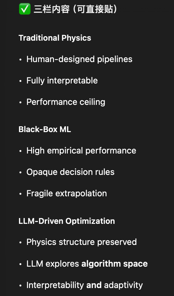
✓ Fully interpretable
✗ Performance ceiling
Human-designed pipelines
Fixed heuristics
Examples:
Matched filtering
χ² tests
✓ High performance
✗ Opaque decisions
End-to-end prediction
Model-centric learning
Examples:
CNNs, DINGO
Algorithms as search objects
Physics-informed objectives
Example:
Evo-MCTS (this work)
AlphaEvolve
Scientific discovery requires interpretability — not just performance.
AI should help us understand why an algorithm works — not just output an answer.
PyCBC (linear-core)
cWB (nonlinear-core)
Simple filters (non-linear)
CNN-like (highly non-linear)
Benchmarking against state-of-the-art methods
(MLGWSC1)
HW, LZ. arXiv:2508.03661 [cs.AI]
LLMs as agents that optimize physics-based algorithms
A new axis: adaptivity over algorithm design
LLMs allow us to search over algorithms, not just over parameters.
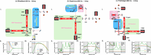
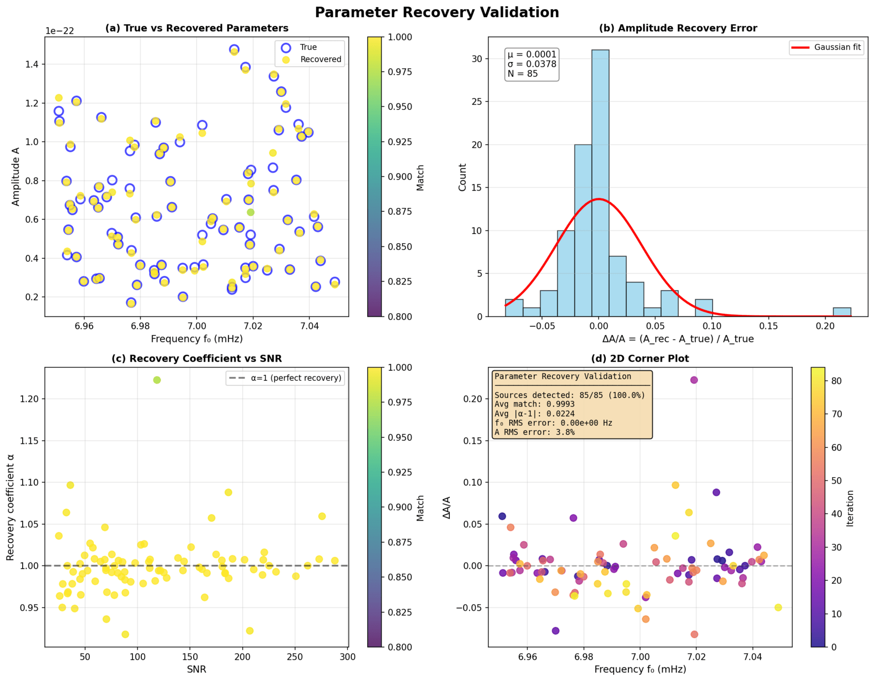
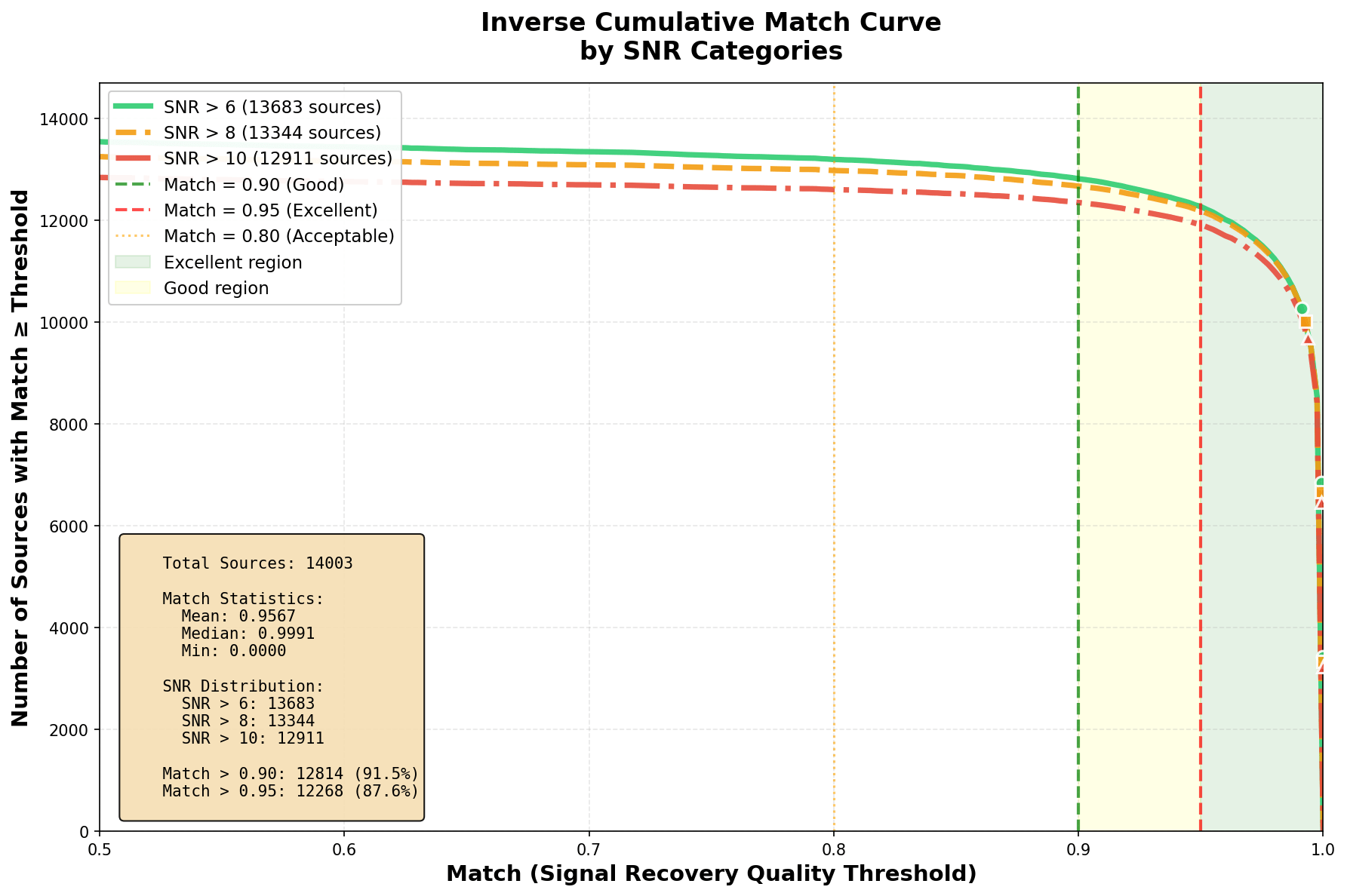
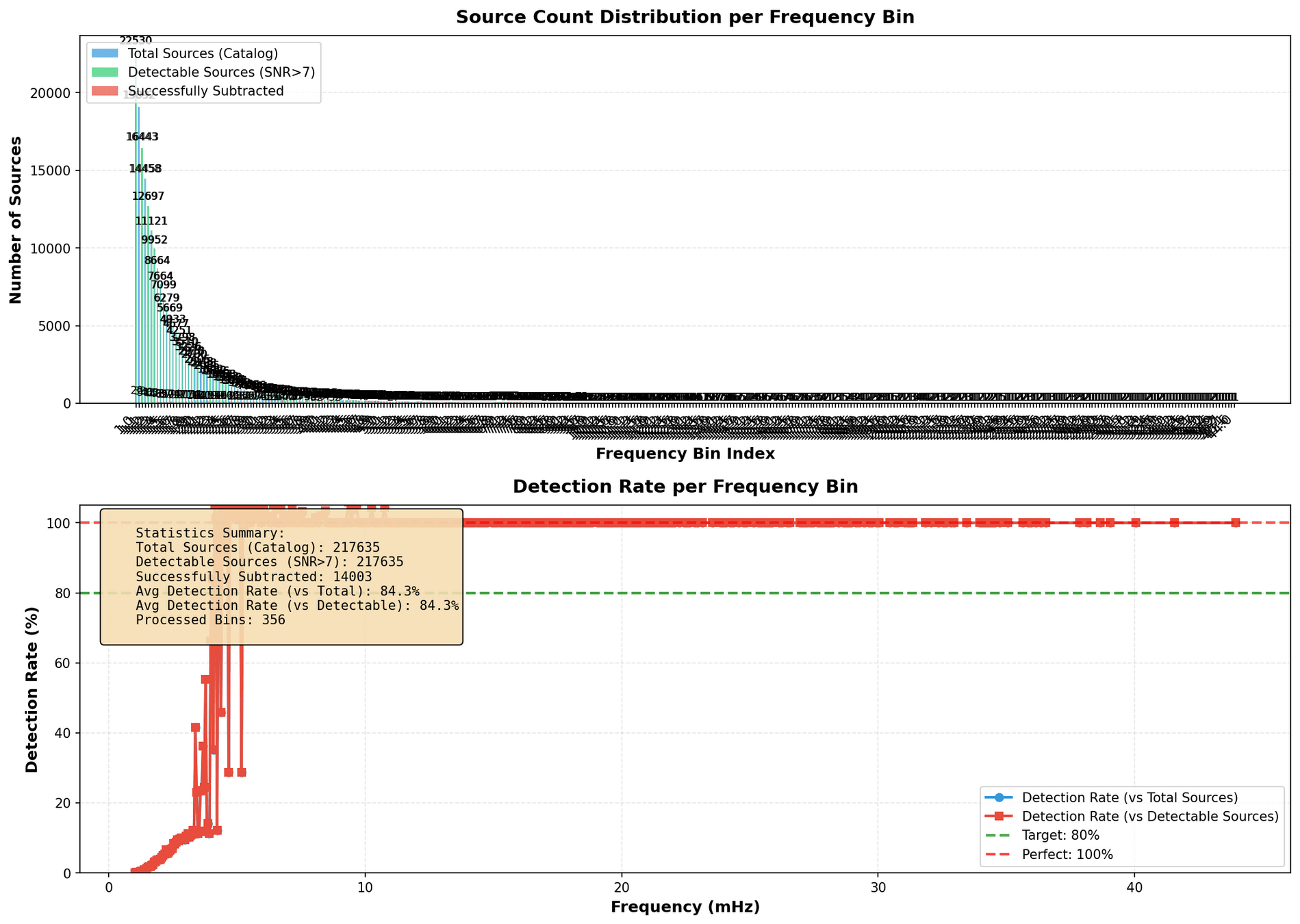
MH Du+, arXiv:2505.16500 [gr-qc]
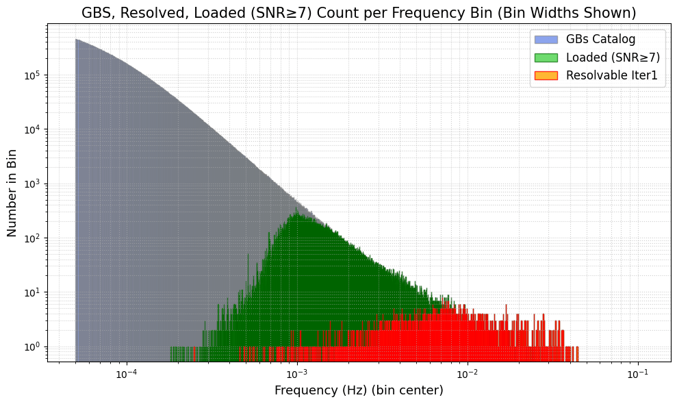
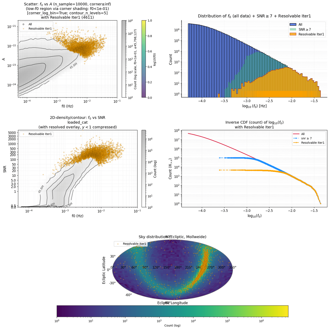
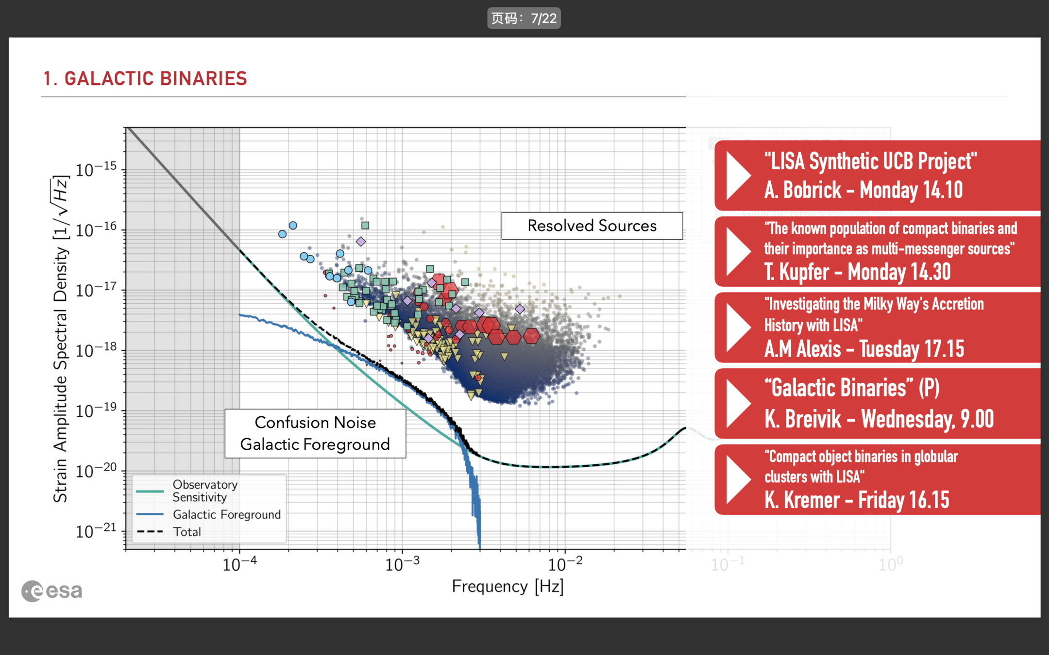
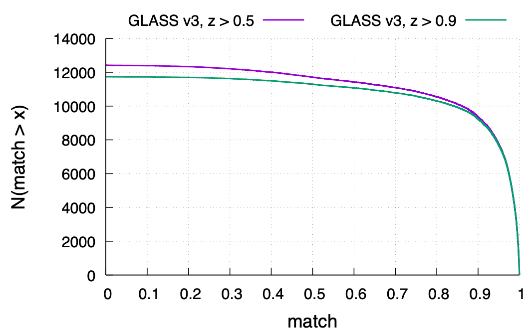
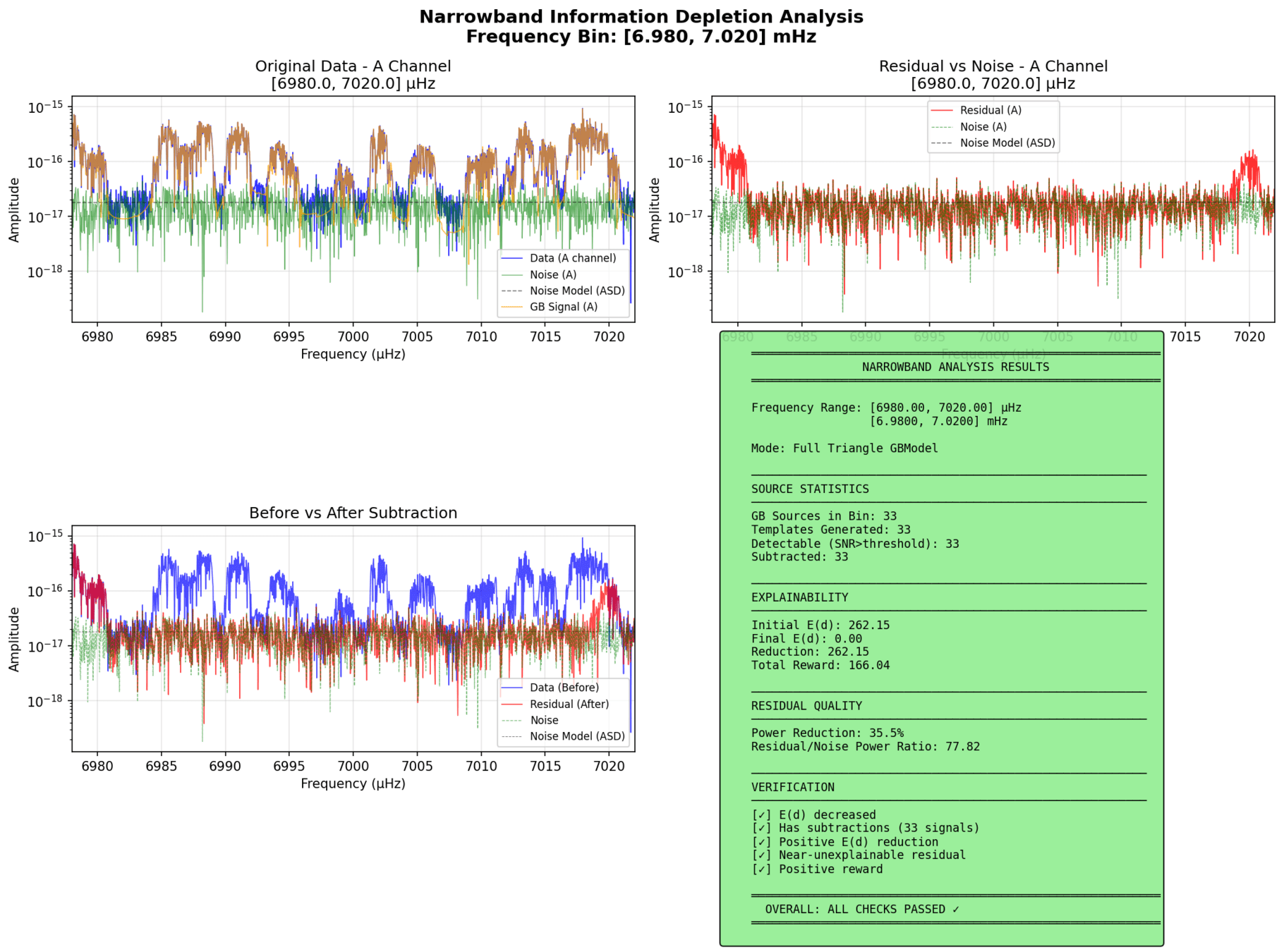
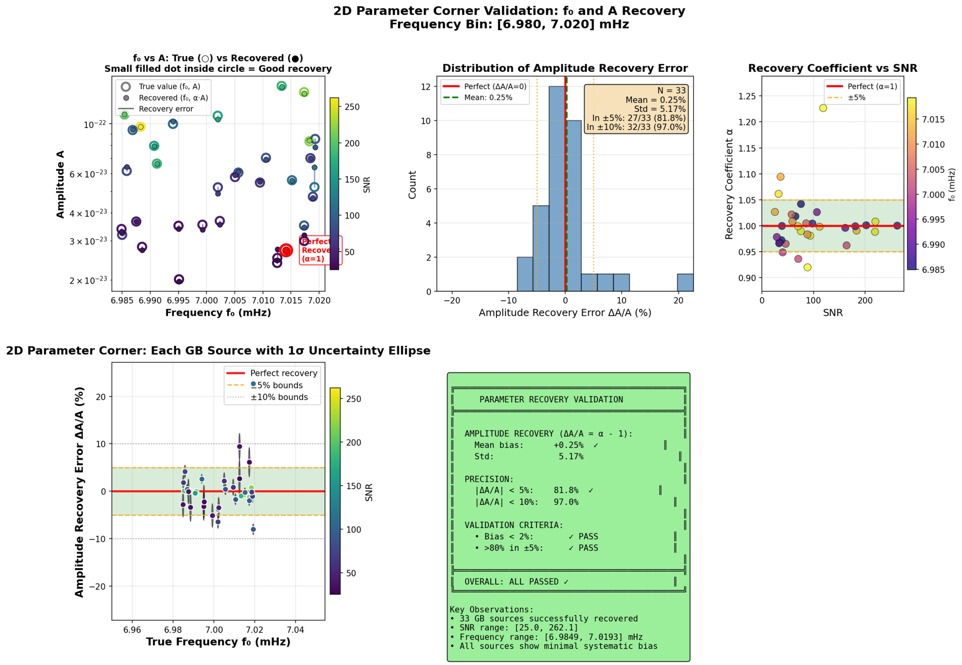
Analyze Non-overlapping Galactic Binaries
The analysis of the best currently known LISA binaries, even making maximal use of the available information about the sources, is susceptible to ambiguity or biases when not simultaneously fitting to the rest of the galactic population. (copied from Littenberg et al. 2404.03046)
credit: Karnesis et al, arXiv:2303.02164v2
credit: M. Katz, The 15th International LISA Symposium
preliminary
preliminary
MH Du+, arXiv:2505.16500 [gr-qc]
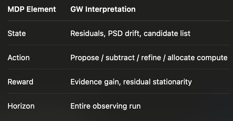
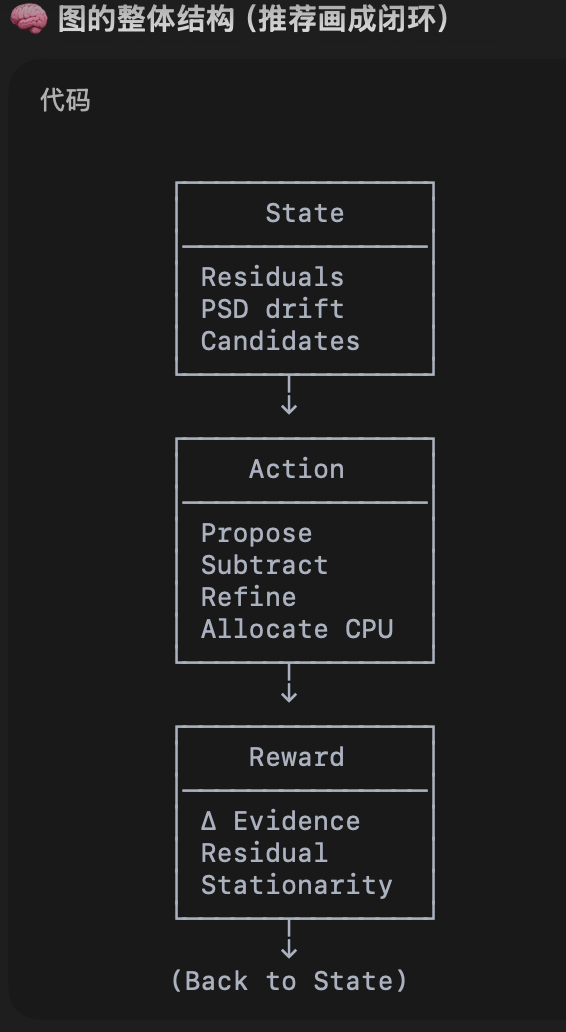
| MDP Element | GW Interpretation |
|---|---|
| State | Residuals, PSD drift, candidate list |
| Action | Propose/subtract/refine/allocate compute |
| Reward | Evidence gain, residual stationarity |
| Horizon | Entire observing run |
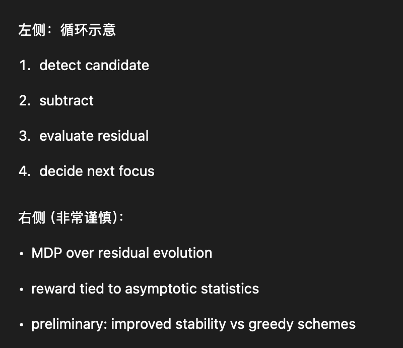
A trajectory tree of global-fitting decisions over time
Nodes: residual states
Edges: modeling actions
(HW+, in preparation)
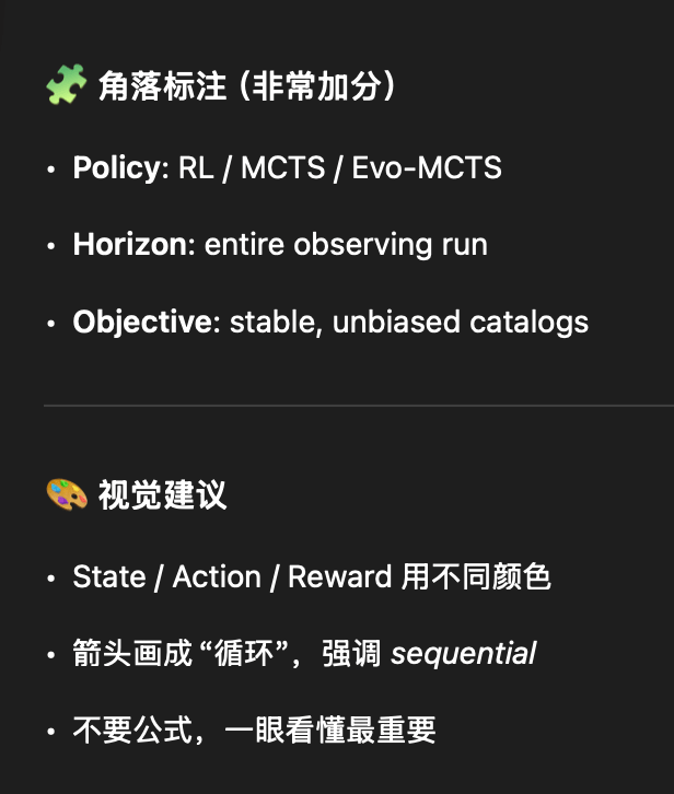
Global fitting as a Markov Decision Process (MDP)
Global fitting is not a single inference — it is a long-horizon control problem.
I don’t claim this is solved. I claim the framing matters.”
preliminary
MH Du+, arXiv:2505.16500 [gr-qc]
A trajectory tree of global-fitting decisions over time
Nodes: residual states
Edges: modeling actions
(HW+, in preparation)
Global fitting is not a single inference — it is a long-horizon control problem.
I don’t claim this is solved. I claim the framing matters.”
See:第八分会场, 5-105
18:00-18:10 张丁锴:Learning Null Channels for Instrumental Noise Characterization in Taiji
preliminary
preliminary
Many GW pipelines already define an MDP — implicitly and inconsistently.
“Once you phrase the problem this way,
RL and MCTS are not exotic — they are obvious.”
for _ in range(num_of_audiences):
    print('Thank you for your attention! 🙏')
空间引力波探测数据仿真及分析春季学习班通知
(第一轮)
空间引力波探测已被列入《国家空间科学中长期发展规划(2024—2050 年)》“时空涟漪”主题下的优先发展方向。为加速形成我国自主的空间引力波探测数据仿真与分析系统,支撑科学目标论证和科学应用系统建设,挖掘和培养青年科研队伍,“空间引力波探测数据仿真及分析春季学习班”将于 2026 年 4 月 23 日-27 日在中国科学院微小卫星创新研究院举办。
太极实验室 2026 年度“大学生创新实践训练计划’
(引力波数据分析与 AI for Science 方向)
中国科学院大学引力波宇宙太极实验室(北京)引力波数据分析与机器学习课题组长期面向全国高校学生开放科研训练机会,现面向全国优秀学生招募参加太极实验室2026年度“大学生创新实践训练计划”,本课题组致力于探索引力波天文学、数值模拟与人工智能技术的交叉研究,重点发展新一代 Al for Science 方法,用于解决复杂物理系统建模、信号处理与科学数据分析问题,欢迎对 引力波科学、人工智能算法与科学计算 充满兴趣的同学加入,在真实科研项目中接受系统训练,并参与国际前沿研究。
for _ in range(num_of_audiences):
    print('Thank you for your attention! 🙏')
Call for Speakers - MLA F2F @ March LVK 2026 (Pisa)
Just a gentle reminder that we’re collecting contributions for the Machine Learning Algorithms (MLA) section!
By He Wang
2026年5月9日 16:00 @内蒙古大学


