Deep Learning Networks & Gravitational Wave Signal Recognization

He Wang (王赫)  

[hewang@mail.bnu.edu.cn]

Department of Physics, Beijing Normal University

In collaboration with Zhou-Jian Cao

July 16th, 2019

Topological data analysis and deep learning: theory and signal applications - Part 4      ICIAM 2019

Outline

• Introduction
  • Background
  • Related works
• ConvNet Model
  • Our past attempts
• ​ MF-ConvNet Model
  • Motivation
  • Matched-filtering in time domain
  • Matched-filtering ConvNet (MF-CNN)
• Experiments & Results
  • Dataset & Training details
  • Recovering GW Events
  • Population property on O1
• Summary

Introduction

• Problems
  • Current matched filtering techniques are computationally expensive.
  • Non-Gaussian noise limits the optimality of searches.
  • Un-modelled signals?

A trigger generator \(\rightarrow\) Efficiency+ Completeness + Informative

Background

• Solution:
  • Machine learning (deep learning)
  • ...

Introduction

• Existing CNN-based approaches:
  • Daniel George & E. A. Huerta (2018)
  • Hunter Gabbard et al. (2018)
  • X. Li et al. (2018)
  • Timothy D. Gebhard et al. (2019)

Related works

Introduction

• Our main contributions:
  • A brand new CNN-based architecture (MF-CNN)
  • Efficient training process (no bandpass, etc.)
  • Effective search methodology (4~5 days on O1)
  • Fully recognized and predicted precisely (<1s) for all GW events in O1/O2

ConvNet Model

• Our past attempts

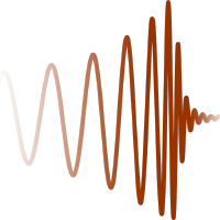
Past attempts on stimulated noise

• The Influence of hyperparameters?

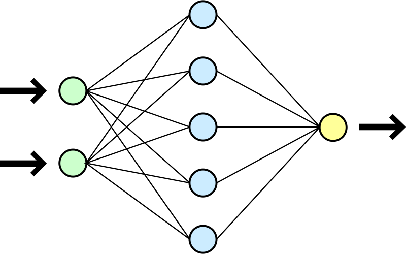
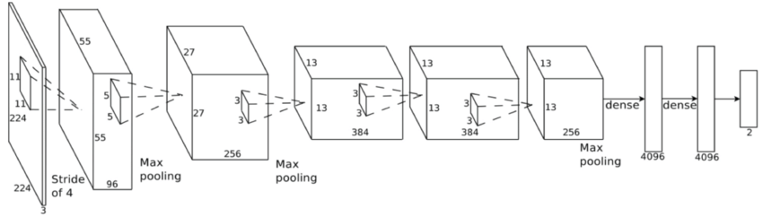
Convolutional neural network (ConvNet or CNN)

Krizhevsky, A., Sutskever, I., & Hinton, G. E. (2012)

ConvNet Model

• The Influence of hyperparameters?

Feature extraction

Merge part

• A glimpse of model Interpretability and Visualization

Convolutional neural network (ConvNet or CNN)

Krizhevsky, A., Sutskever, I., & Hinton, G. E. (2012)

Classification

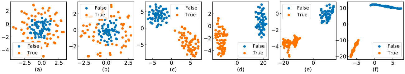
Visualization for the high-dimensional feature maps of learned network in layers for bi-class using t-SNE.

Past attempts on stimulated noise

ConvNet Model

• The Influence of hyperparameters?

Marginal!

Feature extraction

Convolutional neural network (ConvNet or CNN)

Krizhevsky, A., Sutskever, I., & Hinton, G. E. (2012)

Classification

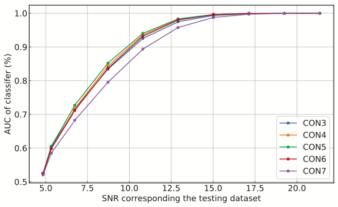
Effect of the number of the convolutional layers on signal recognizing accuracy.

Past attempts on stimulated noise

ConvNet Model

• The Influence of hyperparameters?

Feature extraction

Convolutional neural network (ConvNet or CNN)

Krizhevsky, A., Sutskever, I., & Hinton, G. E. (2012)

Classification

Marginal!

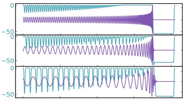
Visualization of the top activation on average at the \(n\)th layer projected back to time domain using the deconvolutional network approach

• A glimpse of model Interpretability using Visualizing

Past attempts on stimulated noise

ConvNet Model

• The Influence of hyperparameters?

Feature extraction

Peak of GW

Convolutional neural network (ConvNet or CNN)

Krizhevsky, A., Sutskever, I., & Hinton, G. E. (2012)

Classification

Marginal!

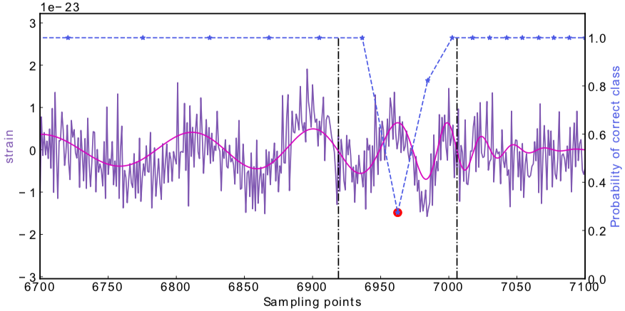
Occlusion Sensitivity

• A glimpse of model Interpretability using Visualizing

Past attempts on stimulated noise

ConvNet Model

• The Influence of hyperparameters?

Feature extraction

Convolutional neural network (ConvNet or CNN)

Krizhevsky, A., Sutskever, I., & Hinton, G. E. (2012)

A specific design of the architecture is needed.

 [as Timothy D. Gebhard et al. (2019)]

Classification

Marginal!

• However, when on real noises from LIGO, this approach does not work that well. (too sensitive + hard to find the events)

Peak of GW

• A glimpse of model Interpretability using Visualizing

Past attempts on stimulated noise

ConvNet Model

MF-ConvNet Model

• Motivation

• Matched-filtering in time domain

• Matched-filtering ConvNet

(In preprint)

Motivation

Matched-filtering (cross-correlation with the templates) can be regarded as a convolutional layer with a set of predefined kernels.

MF-ConvNet Model

Matched-filtering (cross-correlation with the templates) can be regarded as a convolutional layer with a set of predefined kernels.

Is it matched-filtering?

Motivation

MF-ConvNet Model

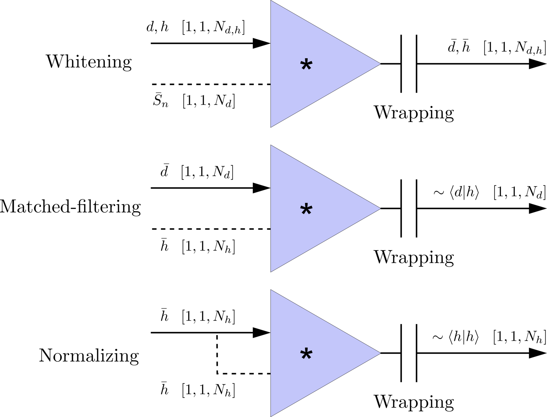
The square of matched-filtering SNR for a given data \(d(t) = n(t)+h(t)\):

Matched-filtering in time domain

Frequency domain

MF-ConvNet Model

(matched-filtering)

(normalizing)

Frequency domain

Time domain

where

(whitening)

\(S_n(|f|)\) is the one-sided average PSD of \(d(t)\)

Matched-filtering in time domain

MF-ConvNet Model

The square of matched-filtering SNR for a given data \(d(t) = n(t)+h(t)\):

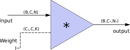
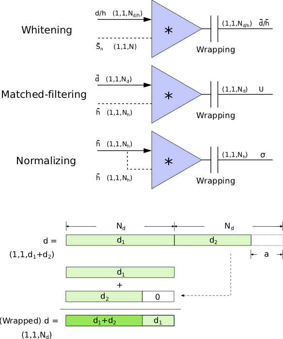
In the 1-D convolution (\(*\)), given input data with shape [batch size, channel, length] :

FYI:       \(N_\ast = \lfloor(N-K+2P)/S\rfloor+1\)

Time domain

(matched-filtering)

(normalizing)

where

(whitening)

Matched-filtering in time domain

MF-ConvNet Model

The square of matched-filtering SNR for a given data \(d(t) = n(t)+h(t)\):

\(S_n(|f|)\) is the one-sided average PSD of \(d(t)\)

（A schematic illustration for a unit of convolution layer)

Time domain

(matched-filtering)

(normalizing)

where

(whitening)

Matched-filtering in time domain

MF-ConvNet Model

The square of matched-filtering SNR for a given data \(d(t) = n(t)+h(t)\):

\(S_n(|f|)\) is the one-sided average PSD of \(d(t)\)

Wrapping (like the pooling layer)

Architechture

\(\bar{S_n}(t)\)

MF-ConvNet Model

\(\bar{S_n}(t)\)

In the meanwhile, we can obtain the optimal time \(N_0\) (relative to the input) of feature response of matching by recording the location of the maxima value corresponding to the optimal template \(C_0\)

Architechture

MF-ConvNet Model

Experiments & Results

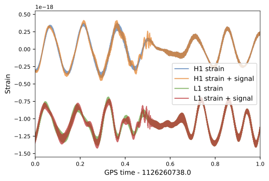
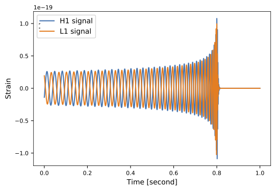
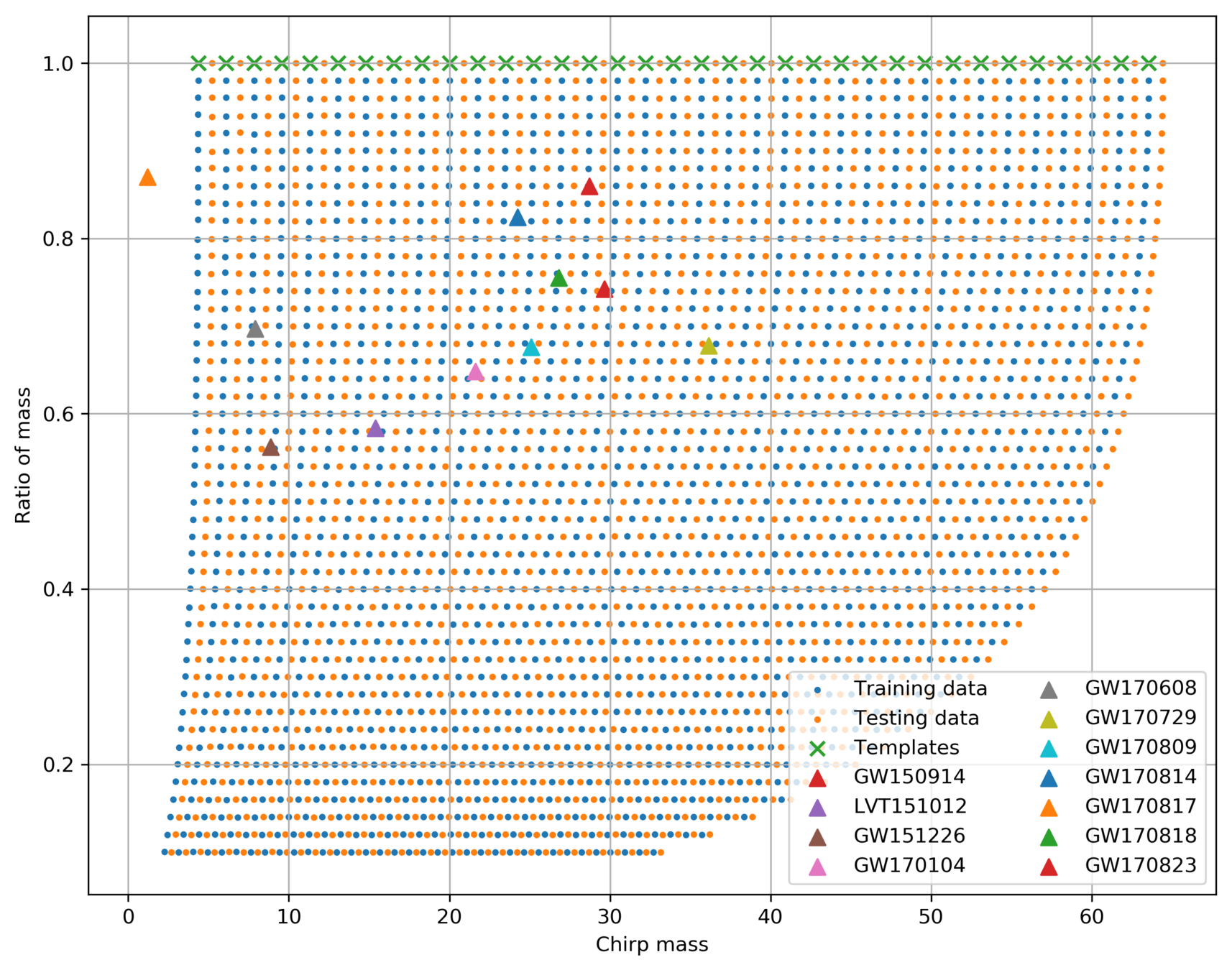
• Dataset & Templates
• Training Strategy
• Search methodology
• Recovering GW Events
• Population property on O1

Experiments & Results

Dataset & Templates

• We use SEOBNRE model [Cao et al. (2017)] to generate waveform, we only consider circular, spinless binary black holes.

FYI: sampling rate = 4096Hz

(In preprint)

• The background noises for training/testing are sampled from a closed set (33*4096s) in the first observation run (O1) in the absence of the segments (4096s) containing the first 3 GW events.

62.50M⊙ + 57.50M⊙ (\(\rho_{amp}=0.5\))

Experiments & Results

Dataset & Templates

(In preprint)

• We use SEOBNRE model [Cao et al. (2017)] to generate waveform, we only consider circular, spinless binary black holes.

• The background noises for training/testing are sampled from a closed set (33*4096s) in the first observation run (O1) in the absence of the segments (4096s) containing the first 3 GW events.

FYI: sampling rate = 4096Hz

Training Strategy

• Tukey window for both data and templates before input the network.
• Xavier initialization [X Glorot & Y Bengio (2010)]
• Binary softmax cross-entropy loss
• Optimizer: Adam [Diederik P. Kingma & Jimmy Ba (2014)]
• Learning rate: 0.003
• Batch size: 16 x 4
• Curriculum learning: decreasing the signal data with SNR \(\rho_{amp}\) distributed at 1, 0.1, 0.03 and 0.02.

• GPUs: 4 NVIDIA GeForce GTX 1080Ti
• MXNet: A Scalable Deep Learning Framework

Probability

(sigmoid function)

Experiments & Results

(In preprint)

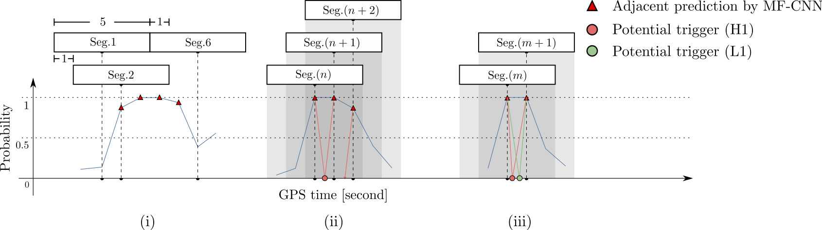
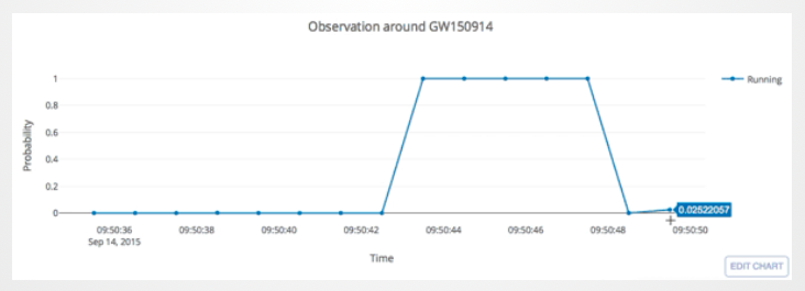
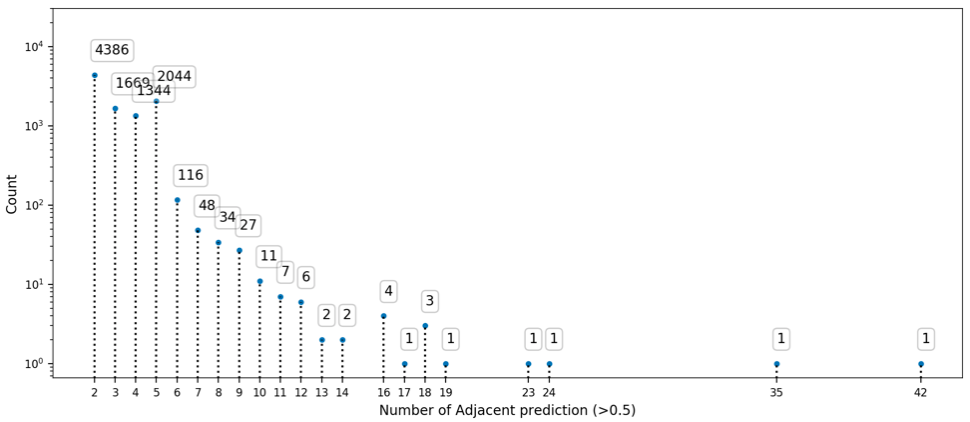
Search methodology

Experiments & Results

(In preprint)

• Every 5 seconds segment as input of our MF-CNN with a step size of 1 second.
• In the ideal case, with a GW signal hiding in somewhere, there should be 5 adjacent prediction for it with respect to a threshold.

Experiments & Results

(In preprint)

• Recovering three GW events in O1

Experiments & Results

(In preprint)

• Recovering three GW events in O1

Experiments & Results

(In preprint)

• Recovering all GW events in O2

Experiments & Results

(In preprint)

• Recovering all GW events in O2

Experiments & Results

(In progress)

Population property on O1

• Sensitivity estimation
  • Background: using time-slides on the closed set from real LIGO recordings
  • Injection: random simulated waveform

Experiments & Results

Population property on O1

(In progress)

• Statistical significance on O1
  • Count a group of adjacent predictions as one "trigger block"
  • For pure background (non-Gaussian), monotone trend should be observed.

Experiments & Results

Population property on O1

(In progress)

• Statistical significance on O1

Experiments & Results

Population property on O1

(In progress)

• Statistical significance on O1

Interesting!

Summary

• Some benefits from MF-CNN architechure

  • Simple configuration for GW data generation

  • Almost no data pre-processing

  • Works on non-stationary background
  • Fast, high acc. on all the events

  • Easy parallel deployments, multiple detectors can be benefit a lot from this design

  • More templates / smaller steps for searching can improve further
  • Rethinking the deep learning neural networks?

Summary

Thank you for your attention!

• Some benefits from MF-CNN architechure

  • Simple configuration for GW data generation

  • Almost no data pre-processing

  • Works on non-stationary background
  • Fast, high acc. on all the events

  • Easy parallel deployments, multiple detectors can be benefit a lot from this design

  • More templates / smaller steps for searching can improve further
  • Rethinking the deep learning neural networks?