


He Wang PRO
Knowledge increases by sharing but not by saving.
He Wang (王赫)
ITP-CAS, Webniar, Aug 13rd, 2020
Based on: PhD thesis (HTML); 10.1103/PhysRevD.101.104003
Abstract:
Deep learning is a neural-inspired pattern recognition technique that is as effective as conventional signal processing. And It has been shown to have considerable potential to identify gravitational-wave (GW) signals. In this talk, I will first review some related works on the detection and characterization of GW signals and some fundamental probabilistic theory of machine learning. I will then present our recent paper (DOI: 10.1103/physrevd.101.104003) about the effect of matched-filtering convolutional neural networks (MFCNN) we proposed on the GW recognition and identifying generalization properties of gravitational waves. At last, I will briefly cover some ongoing works and plans.
Observational Experiment
Theoretical Modeling
Data Analysis
Observational Experiment
Theoretical Modeling
Data Analysis
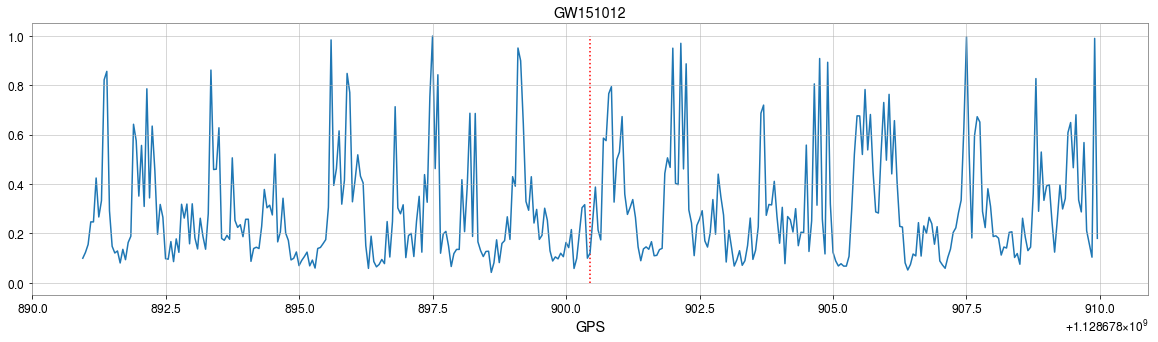
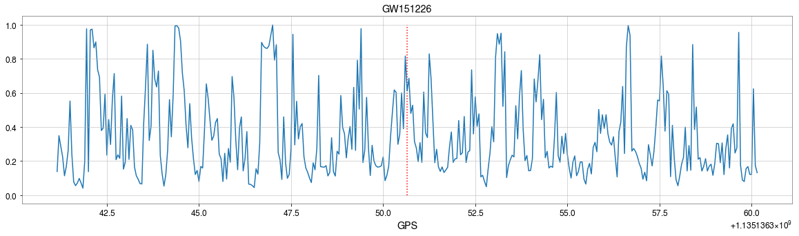
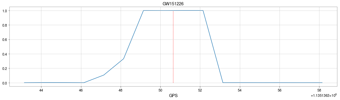
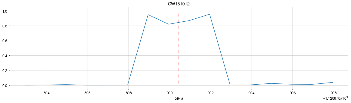
GW151012
GW170729
GW170809
GW170818
GW170823
GW170121
GW170304
GW170721
(GW151205)
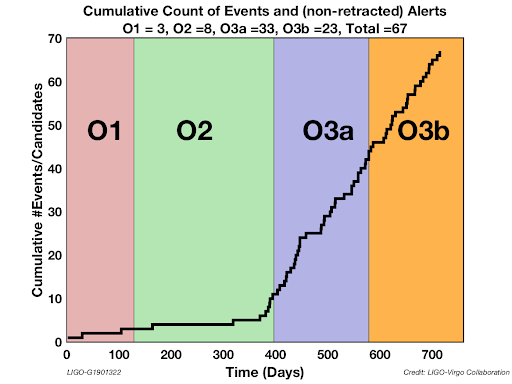
GW Event Detections
O1
O2
O3
GWTC2 (?)
2-OGC (2020)
...
Anomalous non-Gaussian transients, known as glitches
Lack of GW templates
Inadequate matched-filtering method
A threshold is used on SNR value to build our templates bank with a maximum loss of 3% of its SNR.
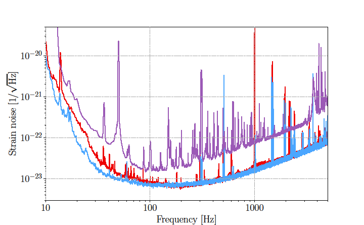
Noise power spectral density
Matched filtering Technique:
Optimal detection technique for templates, with Gaussian and stationary detector noise.
credits G. Guidi
Real-time / low-latency analysis on raw big data
Anomalous non-Gaussian transients, known as glitches
Lack of GW templates
Inadequate matched-filtering method
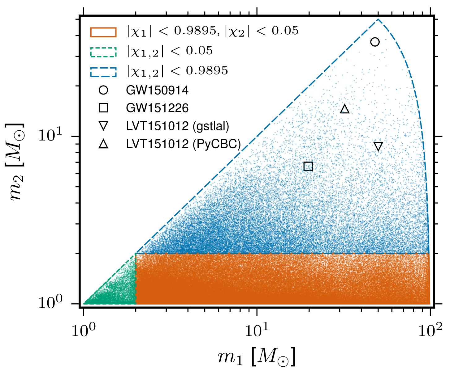
The 4-D search parameter space in O1
covered by the template bank
to circular binaries for which the spin of the systems is aligned (or antialigned) with the orbital angular momentum of the binary.
~250,000 template waveforms are used.
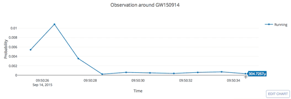
The template that best matches GW150914
Real-time / low-latency analysis on raw big data
Anomalous non-Gaussian transients, known as glitches
Lack of GW templates
Inadequate matched-filtering method
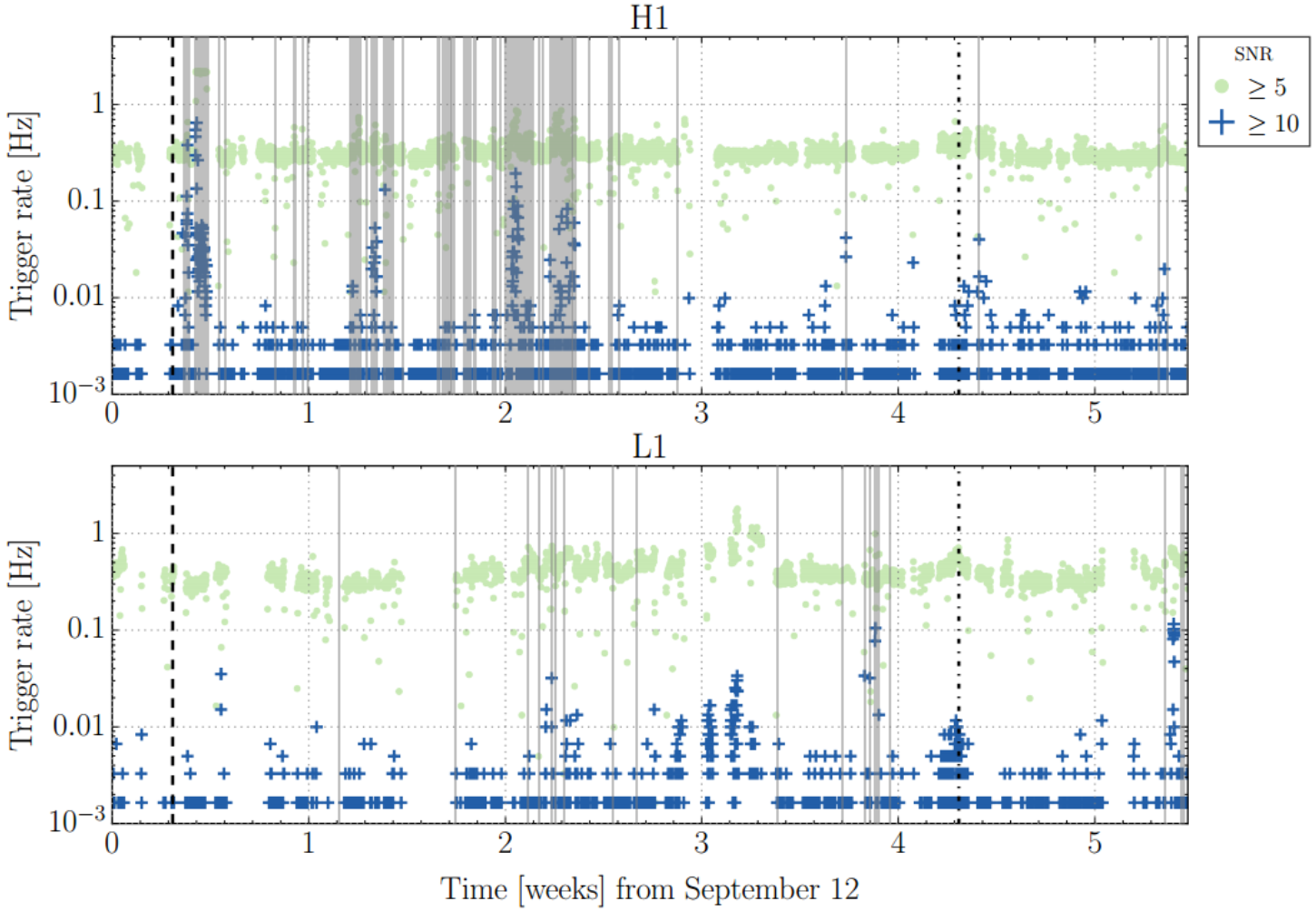
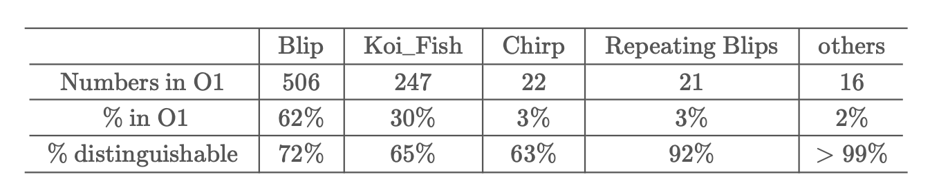
How many "trash" events?
LIGO L1 and H1 triggers rates during O1
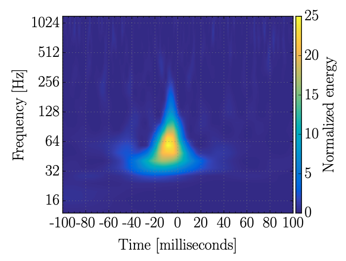
A 'blip' glitch
Real-time / low-latency analysis on raw big data
Anomalous non-Gaussian transients, known as glitches
Lack of GW templates
Real-time / low-latency analysis on raw big data
Inadequate matched-filtering method
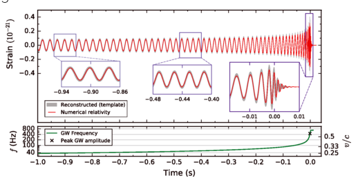
GW170817: Very long inspiral "chirp" (>100s) firmly detected by the LIGO-Virgo network,
GRB 170817A: 1.74\(\pm\)0.05s later, weak short gamma-ray burst observed by Fermi (also detected by INTEGRAL)
First LIGO-Virgo alert 27 minutes later.
Anomalous non-Gaussian transients, known as glitches
Lack of GW templates
Inadequate matched-filtering method
Covering more parameter-space (interpolation)
Automatic generalization to new sources (extrapolation)
Resilience to real non-Gaussian noise (Robustness)
Acceleration of existing pipelines
(Speed, <0.1ms)
...
Why Machine Learning ?
Proof-of-principle studies
Production search studies
Milestones
Real-time / low-latency analysis of the raw big data
More related works, see Survey4GWML (https://iphysresearch.github.io/Survey4GWML/)
"A computer program is said to learn from experience E with respect to some class of tasks T and performance measure P, if its performance at tasks in T, as measured by P, improves with experience E."
Mitchell et al. (1997)
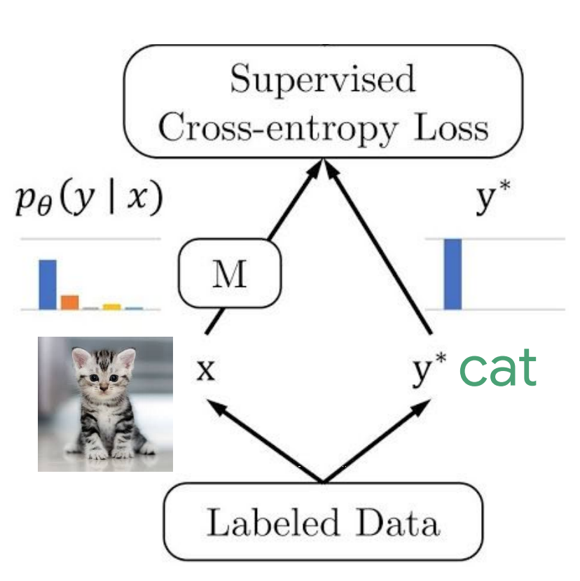
Whether or not a given noisy data contain a GW signal? (classification problem)
The accuracy of classification: the number of correct predictions made divided by the total number of predictions made. (supervised learning)
Characteristic features of GW waveform. (representations learning)
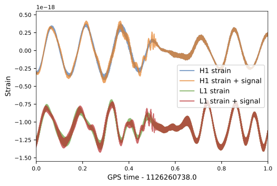
Sampling rate = 4096 Hz
For a GW sample (1 sec): \(n=4096\)
Dataset containing \(N\) examples sampling from true but unknown data generating distribution :
with corressponding ground-truth labels:
Machine learning model is nothing but a map \(f\) from samples to labels:
where \(\mathbb{\Theta}\) is parameters of the model and the outputs are predicted labels:
described by , a parametric family of probability distributions over the same space indexed by \(\Theta\).
Dataset containing \(N\) examples sampling from true but unknown data generating distribution :
Sampling rate = 4096 Hz
For a GW sample (1 sec): \(n=4096\)
with coressponding ground-truth labels:
Machine learning model is nothing but a map \(f\) from samples to labels:
where \(\mathbb{\Theta}\) is parameters of the model and the outputs are predicted labels:
described by , a parametric family of probability distributions over the same space indexed by \(\Theta\).
Objective:
Sampling rate = 4096 Hz
For a GW sample (1 sec): \(n=4096\)
Objective:
to construct cost function (also called loss func. or error func.)
For classification problem, we always use maximum likelihood estimator for \(\Theta\)
FYI: Minimizing the KL divergence corresponds exactly to minimizing the cross-entropy (negative log-likelihood of a Bernoulli/Softmax distribution) between the distributions.
Map / Algorithm
Input
Output
A number
A sequence
Yes or No
Our model / network
Classification
Feature extraction
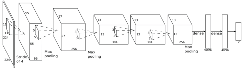
Convolutional neural network (ConvNet or CNN)
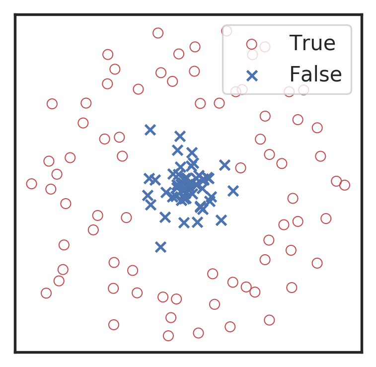
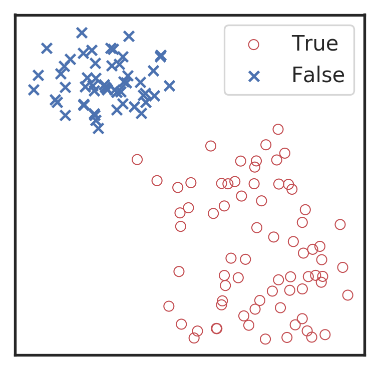
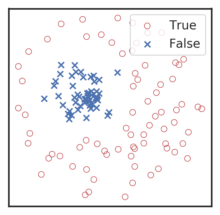
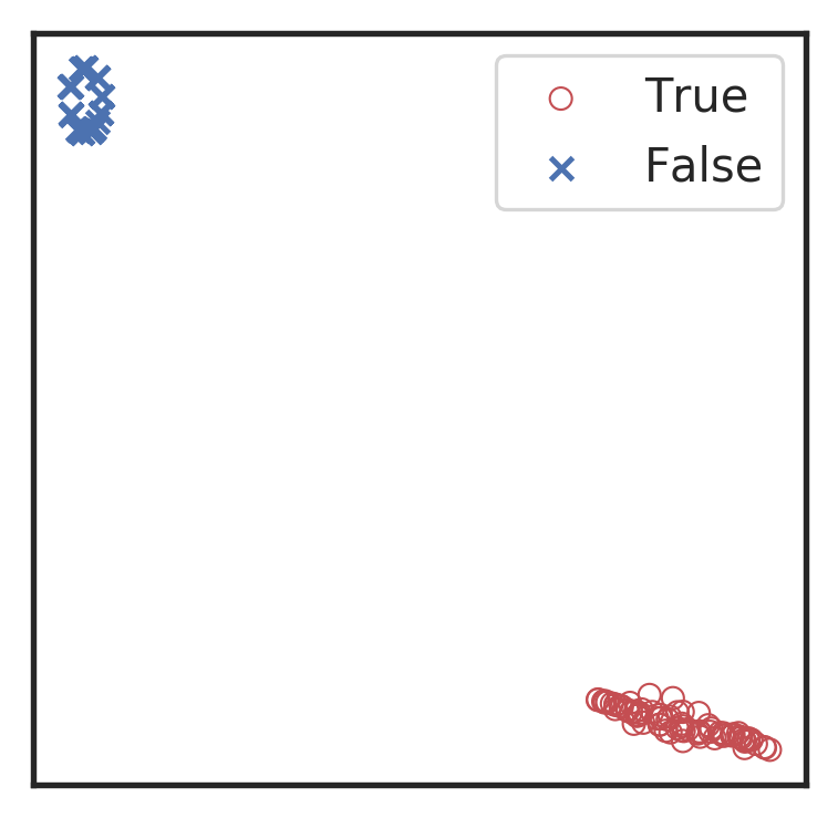
Marginal!
Visualization for the high-dimensional feature maps of learned network in layers for bi-class using t-SNE.
Fine-tune Convolutional Neural Network
Classification
Feature extraction
Convolutional neural network (ConvNet or CNN)
Extracted features play a decisive role.
Visualization of the top activation on average at the \(3\)rd layer projected back to time domain using the deconvolutional network approach
Marginal!
Classification
Feature extraction
Convolutional neural network (ConvNet or CNN)
Extracted features play a decisive role.
Visualization of the top activation on average at the \(3\)rd layer projected back to time domain using the deconvolutional network approach
Marginal!
Classification
Feature extraction
Convolutional neural network (ConvNet or CNN)
Extracted features play a decisive role.
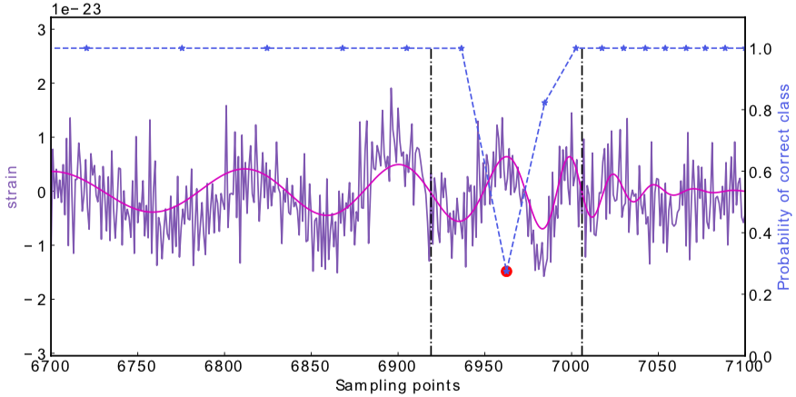
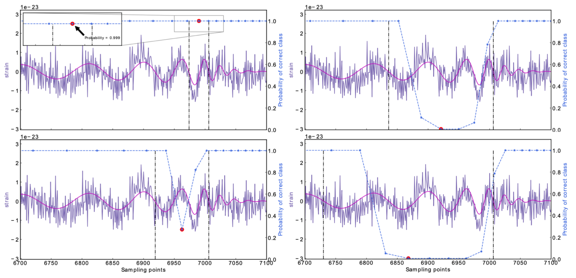
Occlusion Sensitivity
High sensitivity to the peak features of GW.
Marginal!
Classification
Feature extraction
Convolutional neural network (ConvNet or CNN)
Marginal!
Extracted features play a decisive role.
Occlusion Sensitivity
High sensitivity to the peak features of GW.
Classification
Feature extraction
Convolutional neural network (ConvNet or CNN)
A specific design of the architecture is needed.
[as Timothy D. Gebhard et al. (2019)]
(too sensitive against the background + hard to find GW events)
Classification
Feature extraction
Convolutional neural network (ConvNet or CNN)
(too sensitive against the background + hard to find GW events)
A specific design of the architecture is needed.
[as Timothy D. Gebhard et al. (2019)]
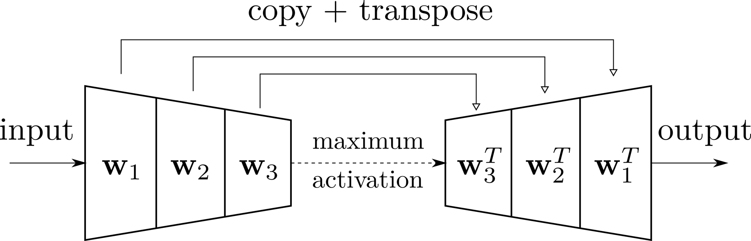
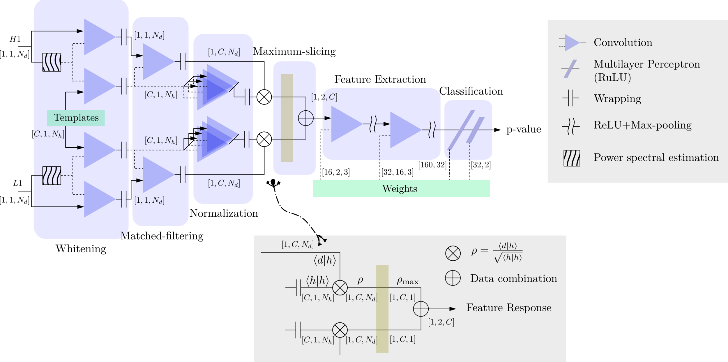
MFCNN
MFCNN
MFCNN
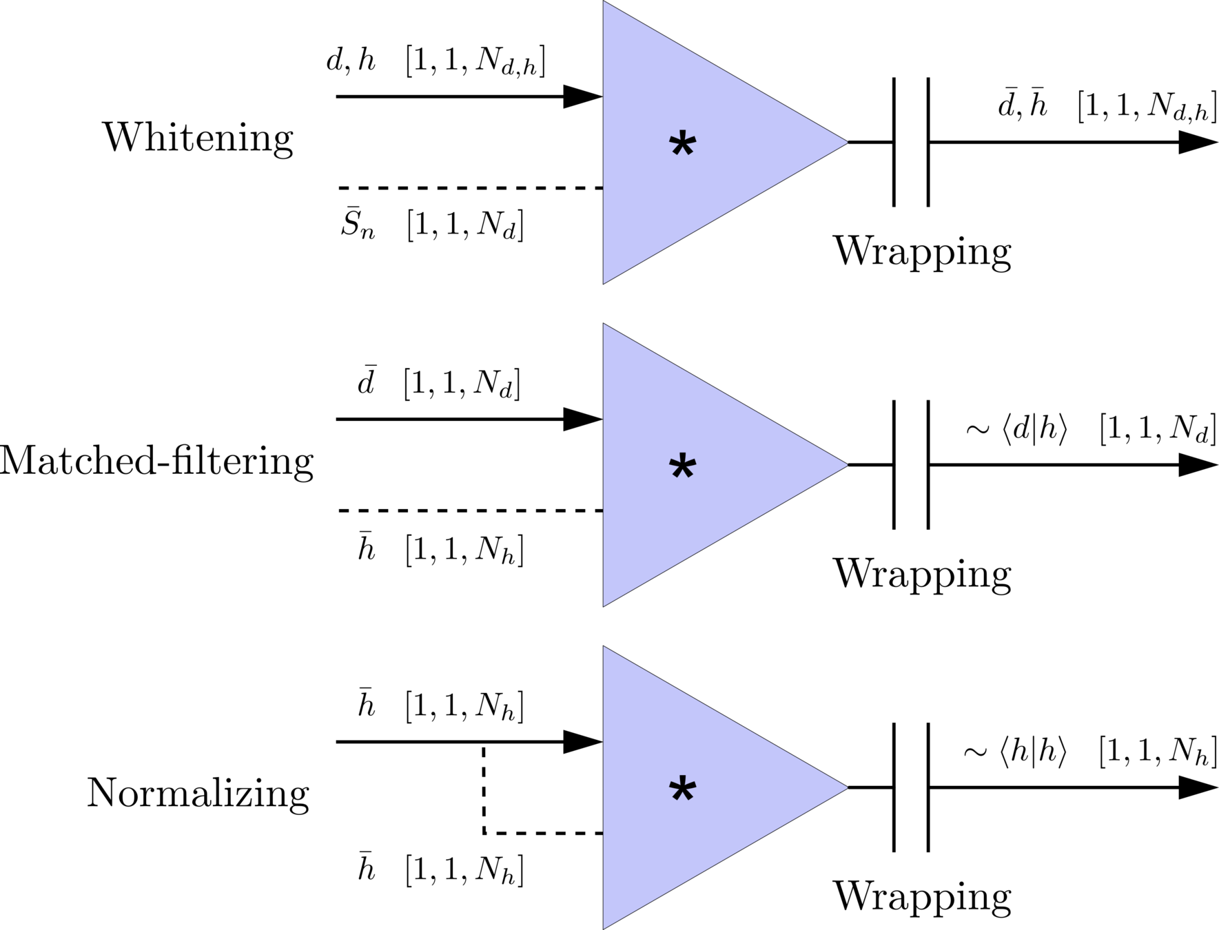
Matched-filtering (cross-correlation with the templates) can be regarded as a convolutional layer with a set of predefined kernels.
>>Is it matched-filtering ?
>>Wait, It can be matched-filtering!
Classification
Feature extraction
Convolutional neural network (ConvNet or CNN)
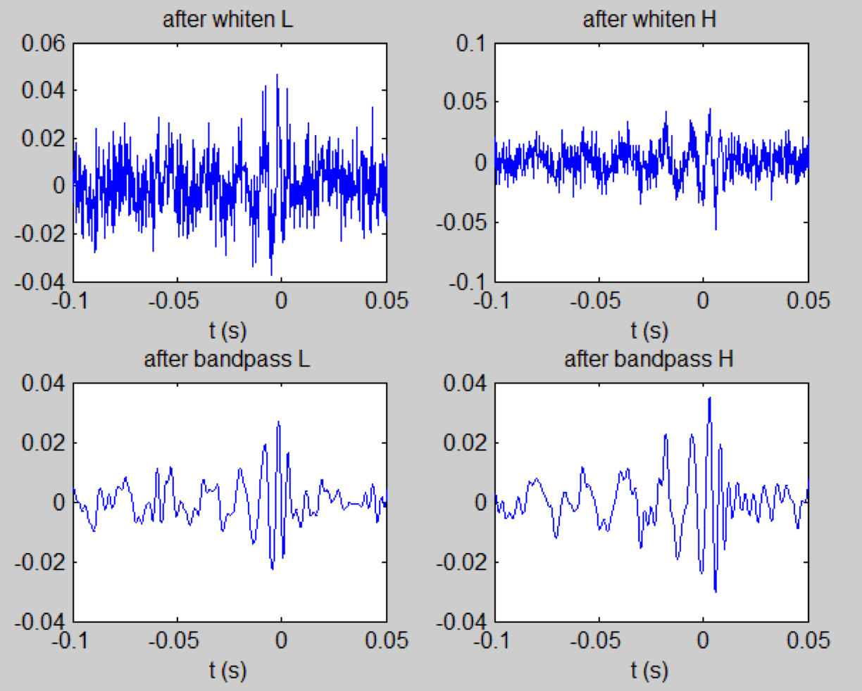
\(S_n(|f|)\) is the one-sided average PSD of \(d(t)\)
(whitening)
where
Time domain
Frequency domain
(normalizing)
(matched-filtering)
\(S_n(|f|)\) is the one-sided average PSD of \(d(t)\)
(whitening)
where
Time domain
Frequency domain
(normalizing)
(matched-filtering)
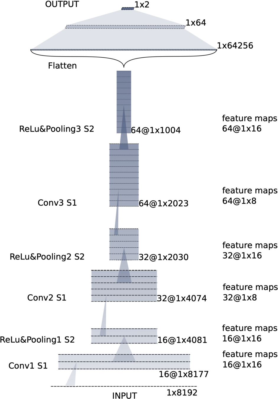
Deep Learning Framework
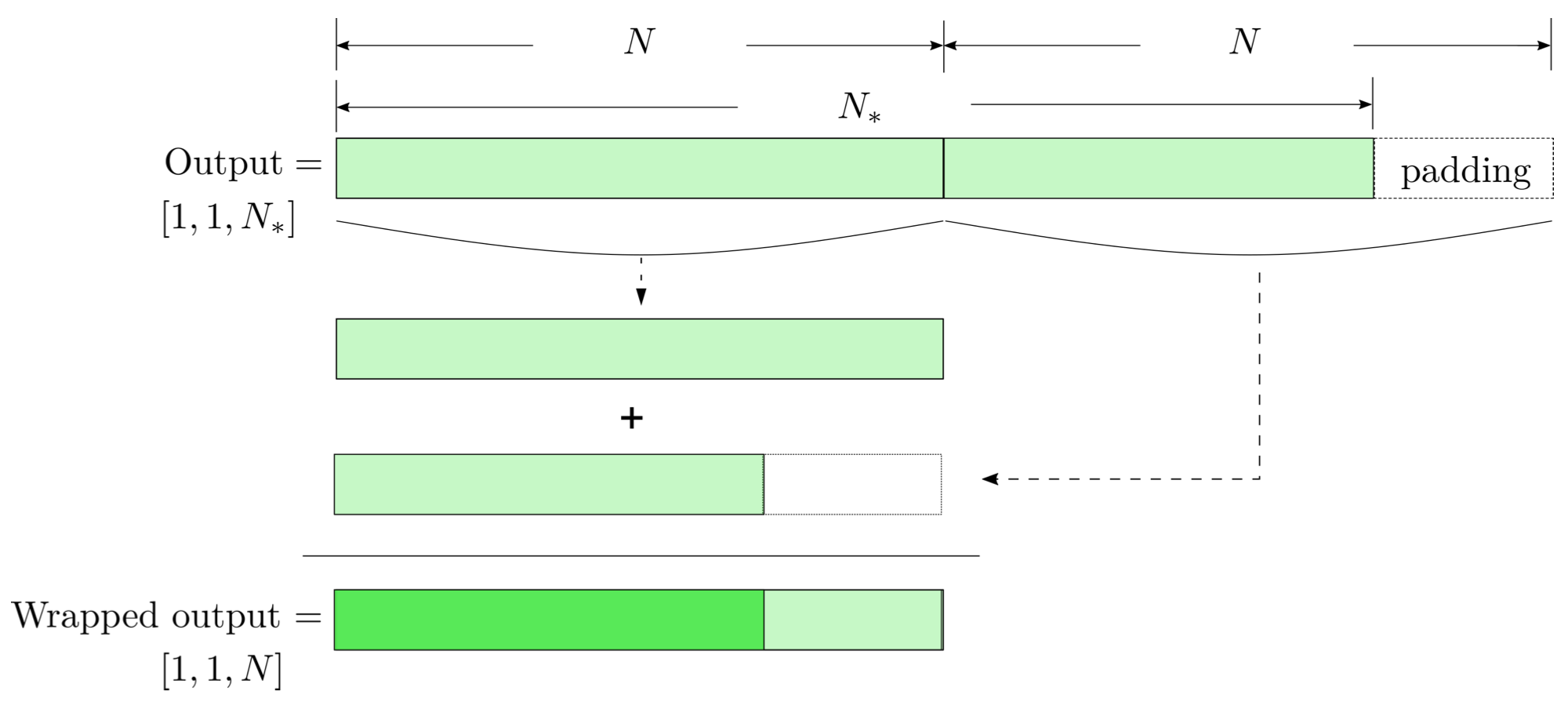
modulo-N circular convolution
\(S_n(|f|)\) is the one-sided average PSD of \(d(t)\)
(whitening)
where
Time domain
Frequency domain
(normalizing)
(matched-filtering)
Deep Learning Framework
modulo-N circular convolution
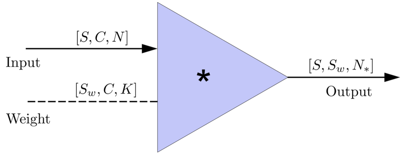
FYI: \(N_\ast = \lfloor(N-K+2P)/S\rfloor+1\)
(A schematic illustration for a unit of convolution layer)
Input
Output
Input
Output
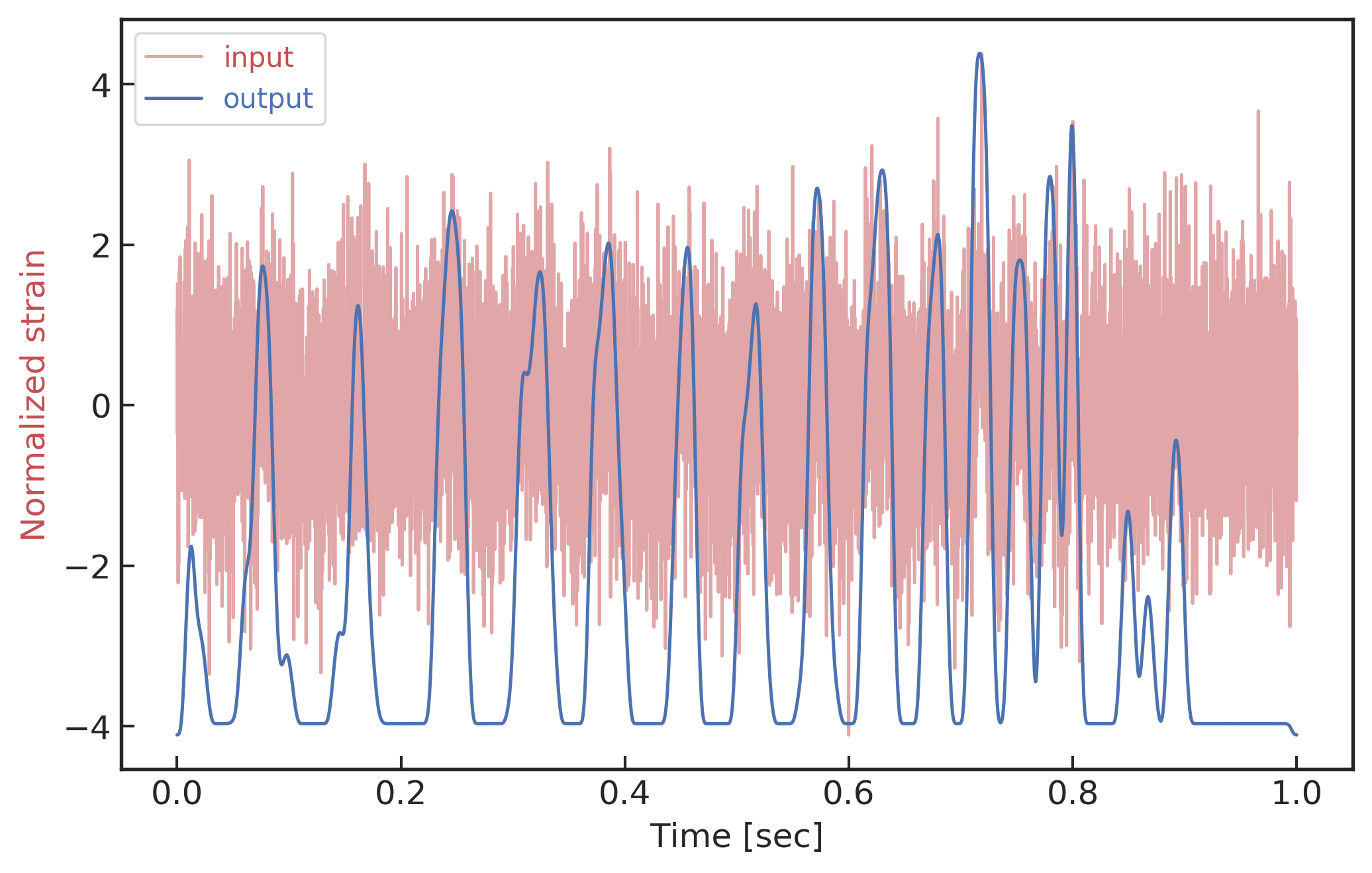
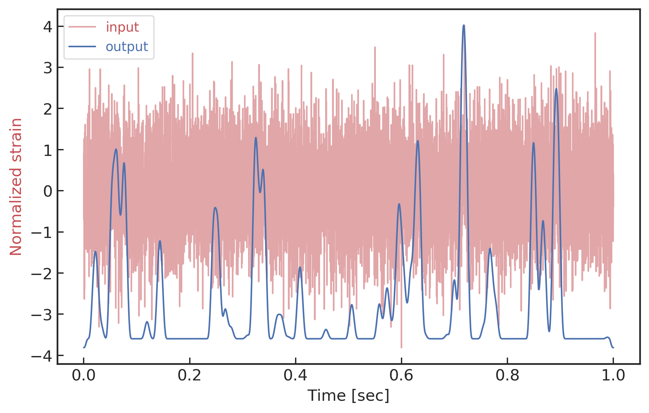
FYI: sampling rate = 4096Hz
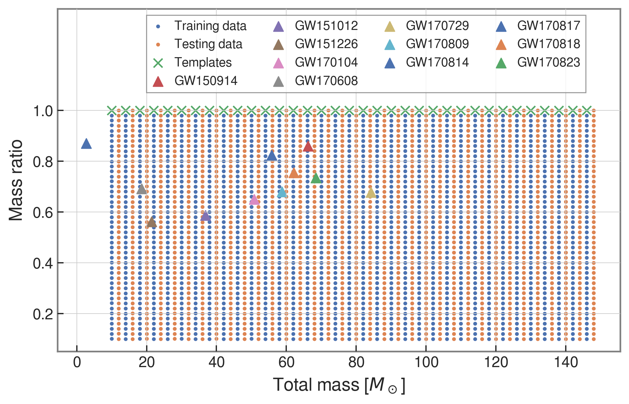
| template | waveform (train/test) | |
|---|---|---|
| Number | 35 | 1610 |
| Length (s) | 1 | 5 |
| equal mass |
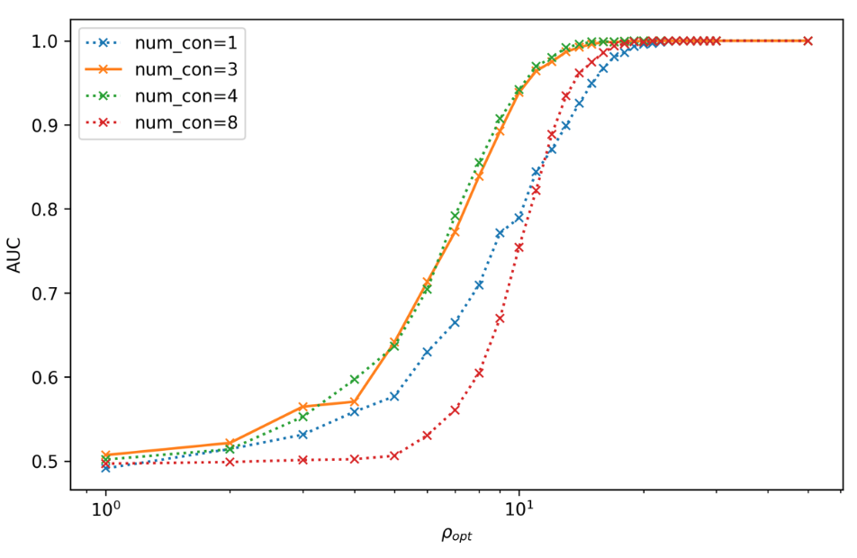
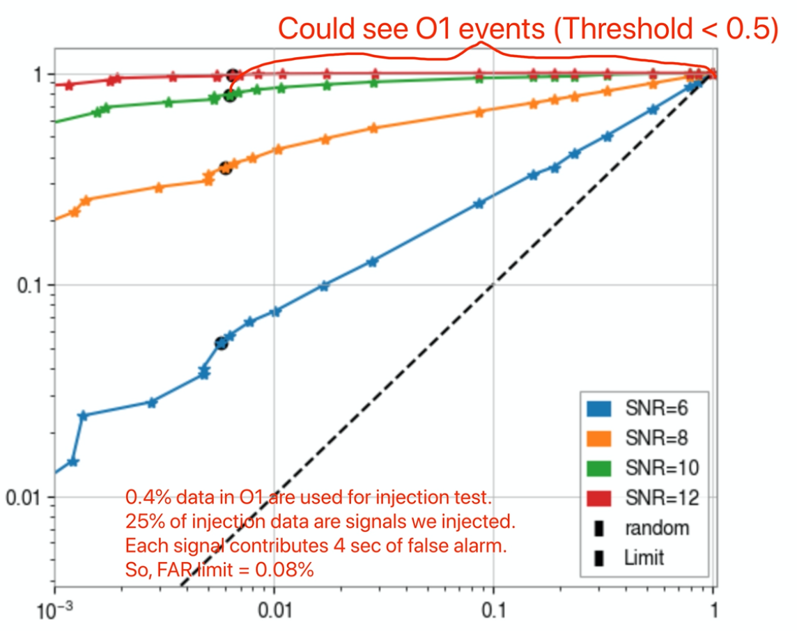
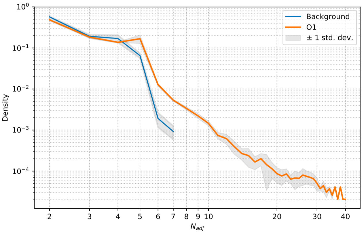
True Positive Rate
False Alarm Rate
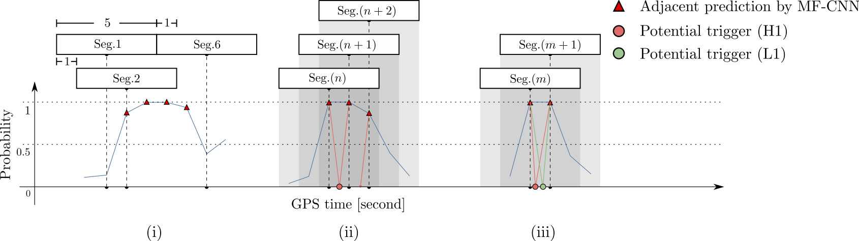
input
Number of Adjacent prediction
a bump at 5 adjacent predictions
Some benefits from MF-CNN architecture:
Simple configuration for GW data generation and almost no data pre-processing.
Easy parallel deployments, multiple detectors can benefit a lot from this design.
Parameter estimation (the current “holy grail” of machine learning for GWs.)
Machine learning search for continuous GWs \(\rightarrow\) space-based detector.
An improved MFCNN for:
higher sensitivity
lower FAR (a metric for estimation is urgently needed)
and more kinds of GW sources, other than CBC.
2008.03312
By He Wang
ITP-CAS, Webniar, Aug 13rd, 2020


