A Theory of Cluster Patterns in Tensors
2025 James B. Wilson

https://slides.com/jameswilson-3/cluster-patterns-theory/
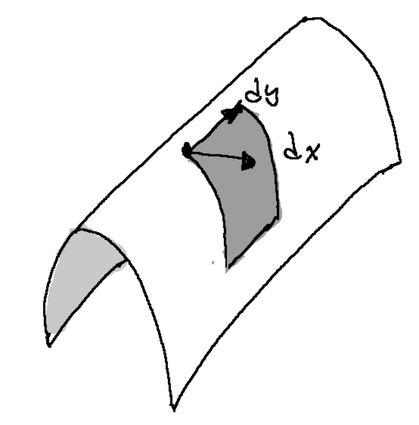
Tensors as area & volume
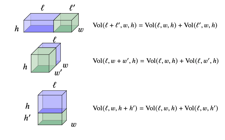
Volume basics
\[Vol(\ell, w,h)= \ell\times w\times h\]
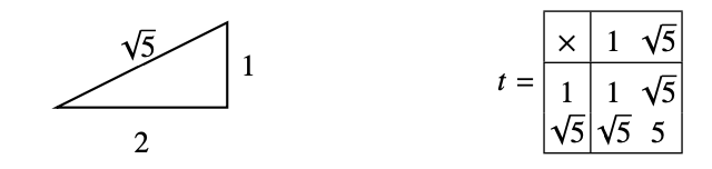
Volume reality
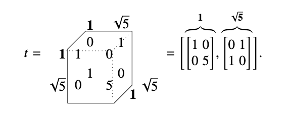
\[Vol(t\mid \ell, w,h)= t\times \ell\times w\times h\] where \(t\) converts miles/meters/gallons/etc.
tensor conversion
Miles
Yards
Feet
Gallons
Area...easy
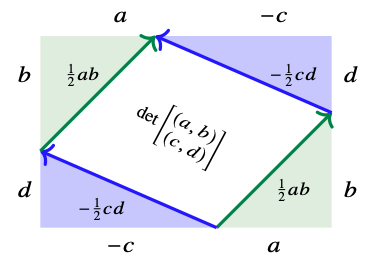
Area...not so easy
\[det\left(\begin{array}{c} (a,b)\\ (c,d)\end{array}\right) = ad-bc\]
\[= \begin{bmatrix} a & b\end{bmatrix}\begin{bmatrix} 0 & 1 \\ -1 & 0 \end{bmatrix}\begin{bmatrix} c\\ d \end{bmatrix}\]
tensor
Tensor's as Multiplication Tables
Notation
\[a*e*\cdots *u\qquad [u,v]\qquad a\otimes e\otimes \cdots \otimes u\] \[[a,e,\ldots, u]\qquad \langle a,e,\ldots, u\rangle\]
Choose a heterogenous product notation
Choose index yoga, mine is "functional", i.e. \(v\in \prod_{a\in A} U_a\)
\[\langle v\rangle =\langle v_1,\ldots, v_{\ell}\rangle= \langle v_a,v_{\bar{a}}\rangle\qquad \{1,\ldots,\ell\}=\{a\}\sqcup\bar{a}\]
When explicit tensor data \(t\)
\[\langle t\mid v\rangle =\langle t \mid v_B,v_C\rangle \qquad A=B\sqcup C\]
\(v\in \prod_{a\in A} V_a\) means \(v:A\to \bigcup_{a\in A} V_a\) with \(v_a\in V_a\).
\(v_B\) is restriction of the function to \(B\subset A\)
\((v_B,v_C)\) is disjoint union of functions \(B\sqcup C\to \bigcup_{e\in B\sqcup C} V_e\)
Technical Requirements
Each space \(V_a\) needs a suite of (multi-)sums
Product commutes with sums ("Distribution/Multi-additive")
\(\displaystyle \int_I v_a(i) d\mu\) could be various sum algorithms "sum(vs[a],method54)"
For \(\{v_a(i)\mid i\in I\}\)
\[\int_I \langle v_a(i),v_{\bar{a}}\rangle\,d\mu = \left\langle \int_I v_a(i)\,d\mu,v_{\bar{a}}\right\rangle\]
Sums are entropic/Fubinian
\[\int_I \int_J f\, d\mu d\nu=\int_J\int_I f \, d\nu d\mu\]
Theory
TL;DR tensors behave like your algebra teacher told you (almost).
Murdoch-Toyoda Bruck
All entropic sums that can solve equations \(a+x=b\) are affine.
Eckmann-Hilton
Entropic sums with 0 are associative & commutative.
Grothendieck
You can add negatives.
Mal'cev, Miyasnikov
You can enrich distributive products with universal scalars.
Davey-Davies
Tensor algebra is ideal determined precisely for affine.
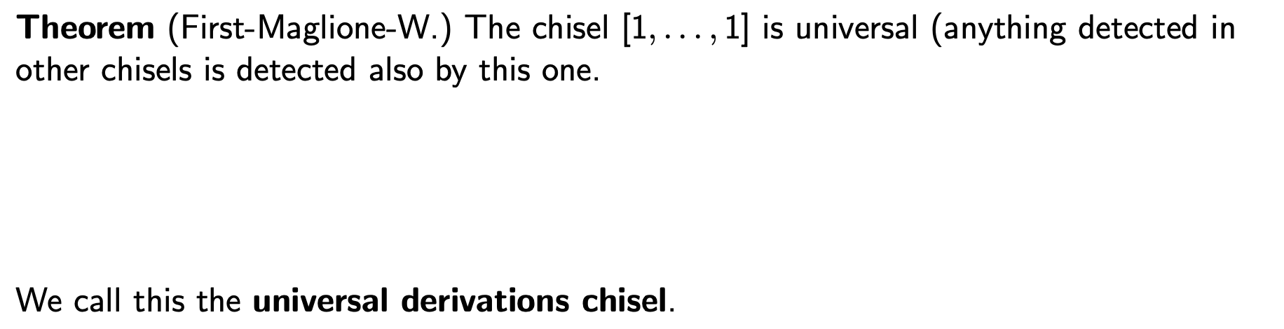
First-Maglione-Wilson
Full classification of algebraic enrichment:
- If 3 or more positions must be Lie
- 2 can be associative or Jordan.
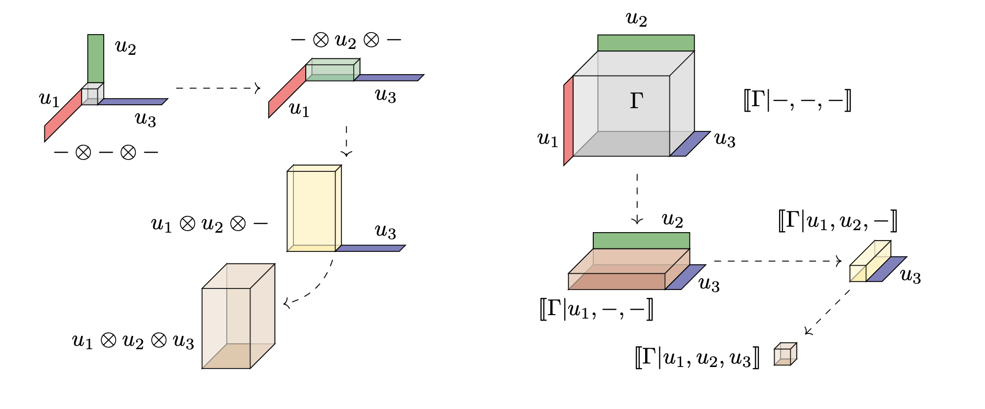
Illustrating Tensor Product/Contraction
(Aka. Inner/Outer products, Co-multiply/Multiply)
Inflate: data of product stored as a bigger array.
Contract: integral of data stored in smaller array.
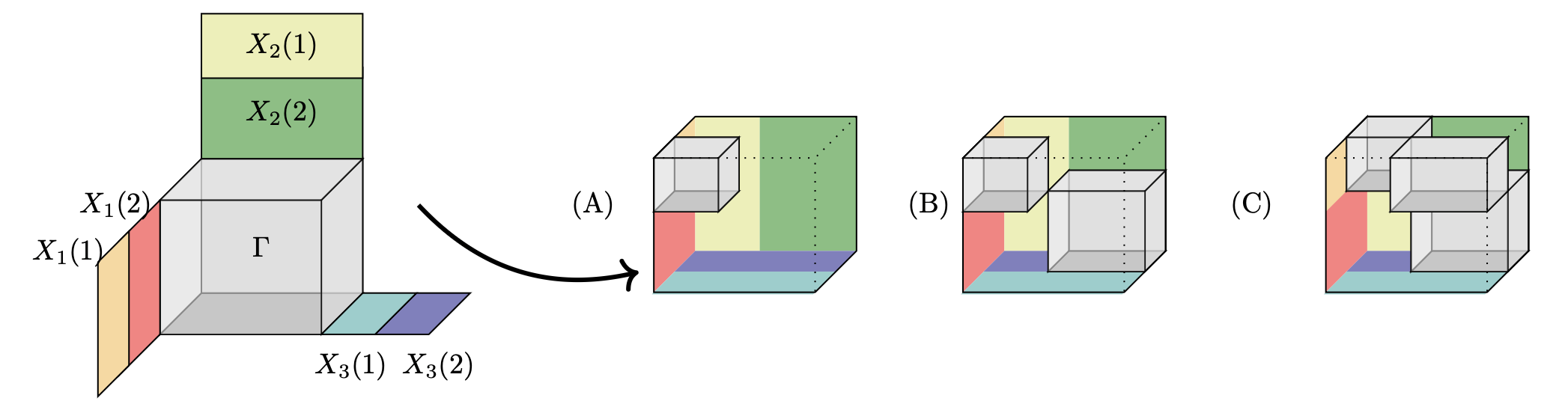
Illustrating manipulating tensors
-
Shaded gray illustrates possibly non-zero
-
A basis of vectors contracted on each side stacks up contractions to reconstitute a new tensor.
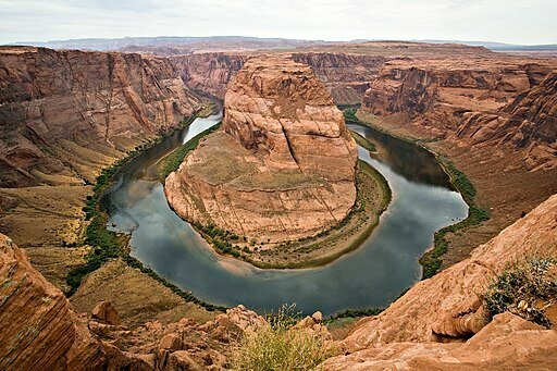
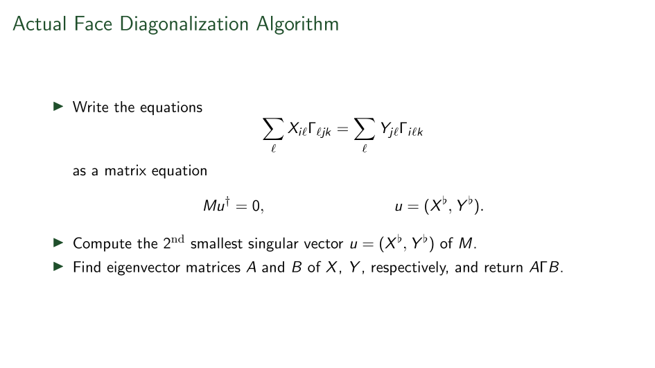
New uses? Sales Volume?
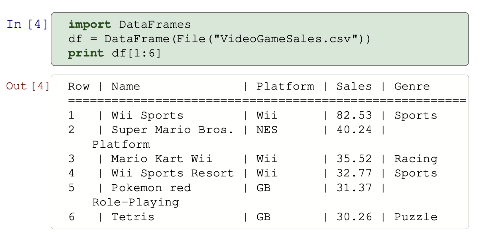
Data science tensors
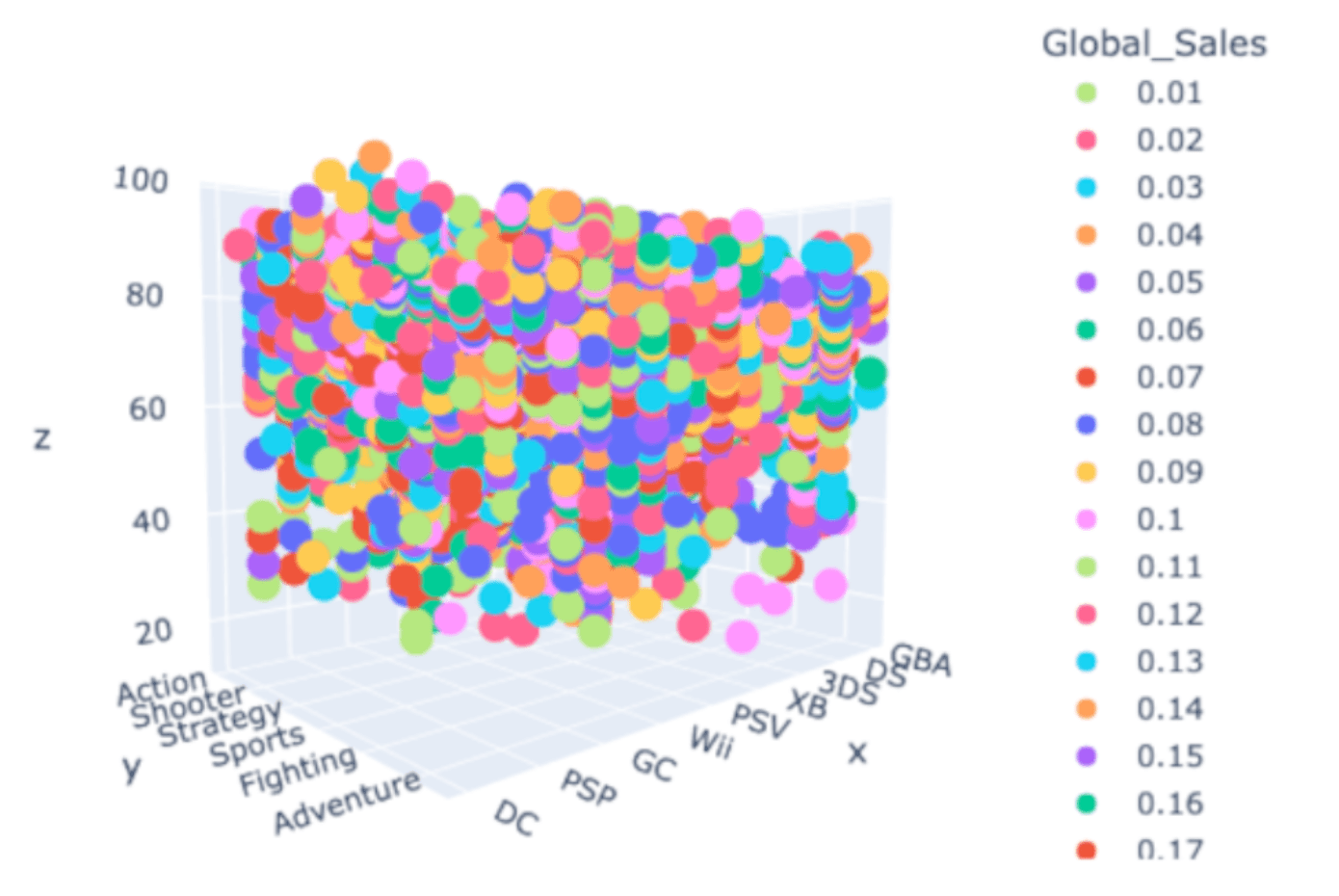
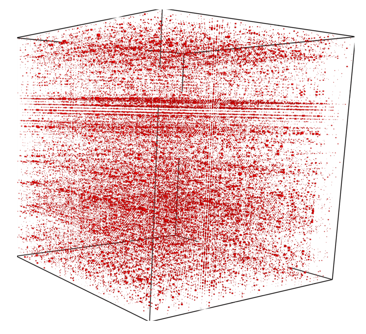
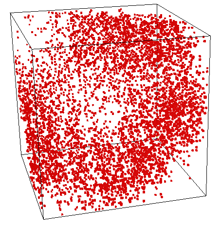
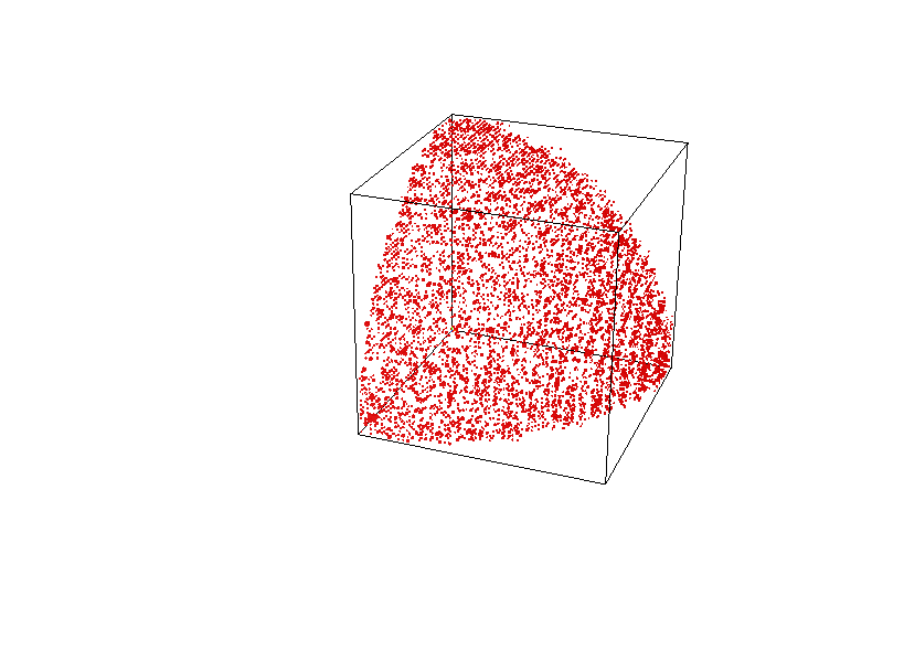
Histogram Visualization
What we have found is computable.
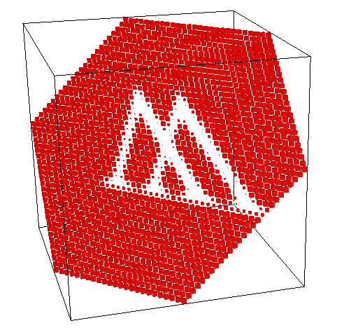
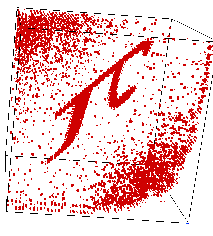
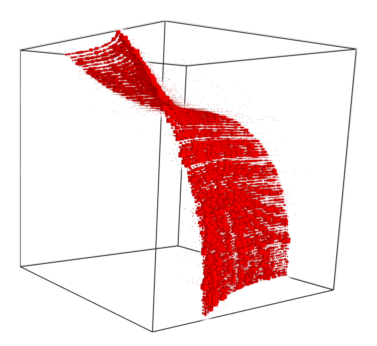
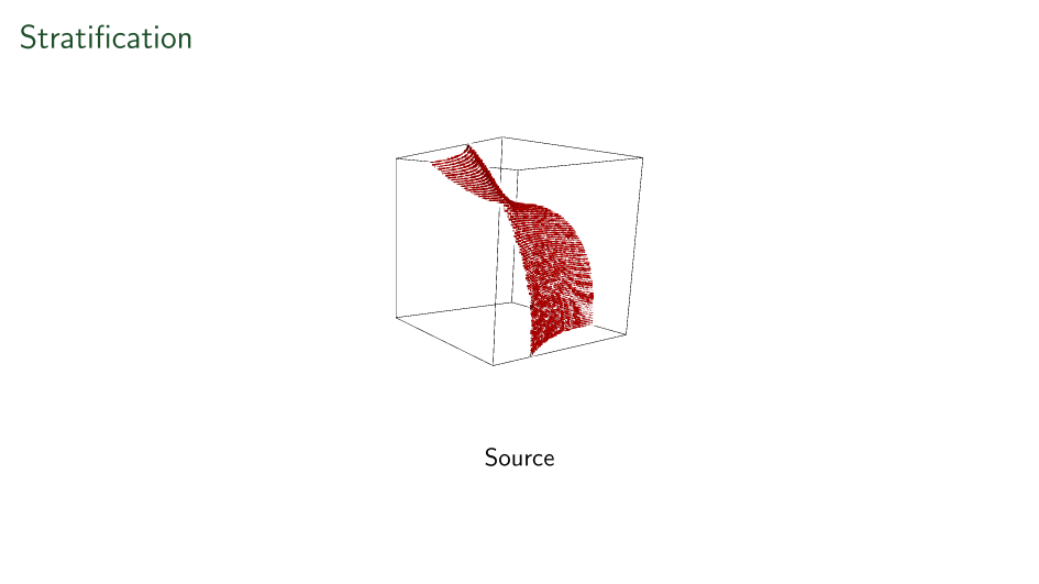
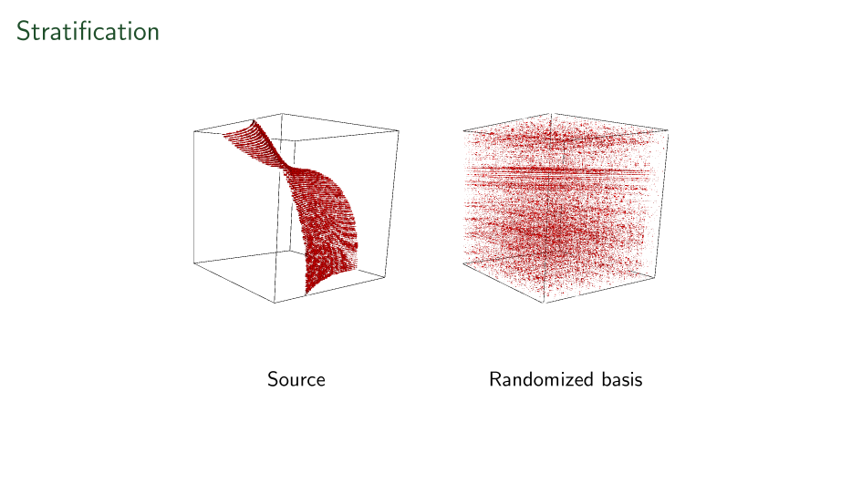
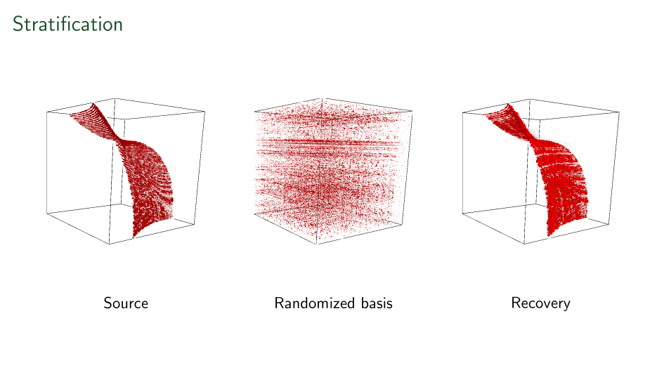
"Random" Basis Change
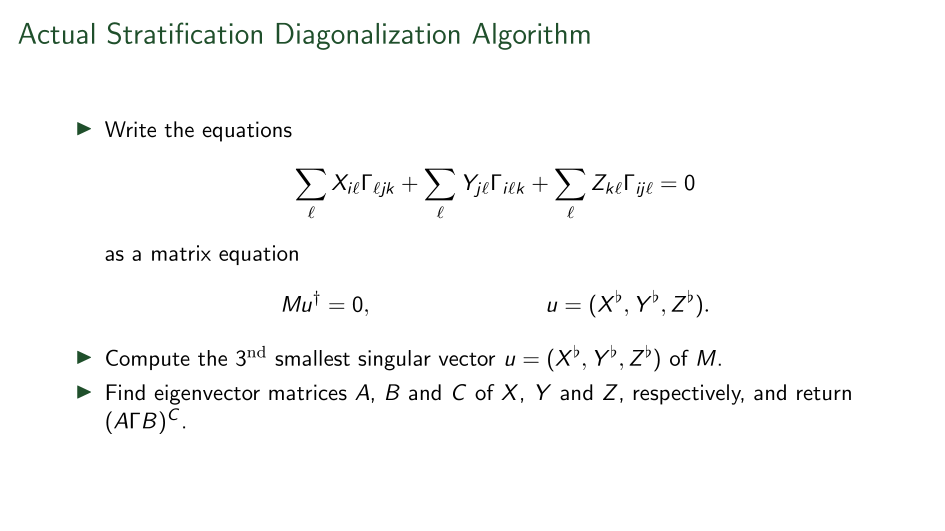
Our blind source separation
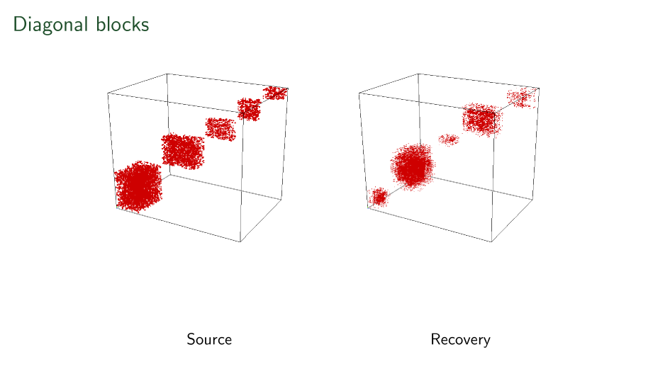
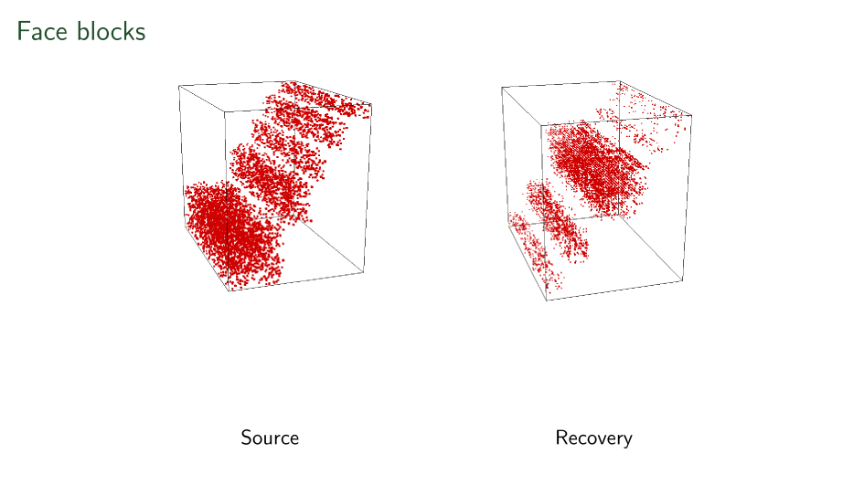
First ever stratification
Shown here is a linear-time recovered unique basis change applied to each side of a tensor to make it's support on a surface.
Blocks have been seen before
- Mal'cev folklore credited by numerous Russian papers.
- Miyasnikov in Model Theory Tensors
- Cardoso 1991 Statistical tensors
- Eberly-Geisbrecht 2000 Algebraic tensors
- Acar et. al. 2005 Data science
- W. 2007/8 Central/Direct products of p-groups
-
Maehara and K. Murota, 2010.
- Lathauwer 2008 Small rank cases
- 2024+ Liu-Maglione-W. \(O(d^{1.5\omega+n})\)-time solution (n=valence, d=max dimension, \(\omega\)=matrix mult. exp.).
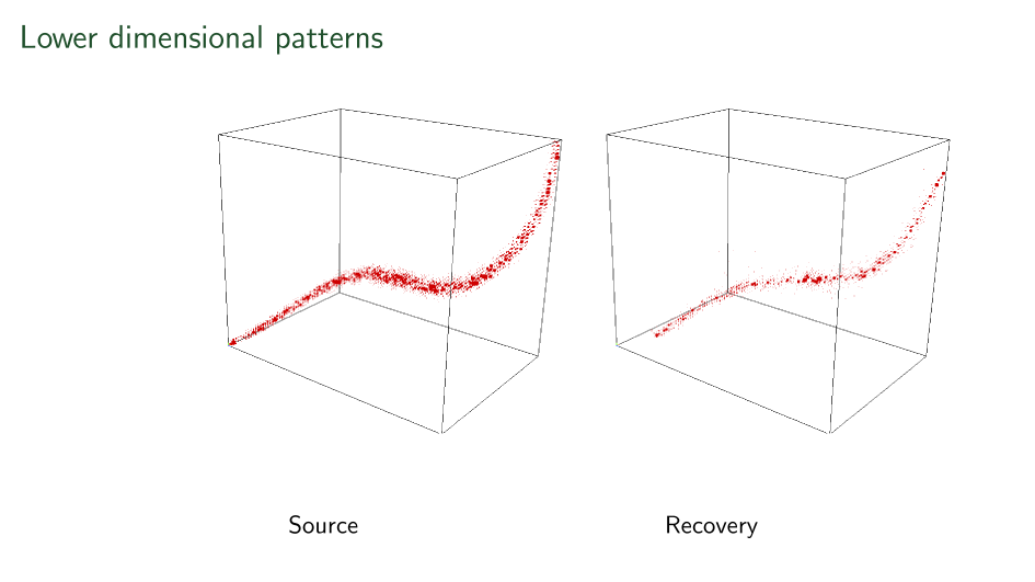
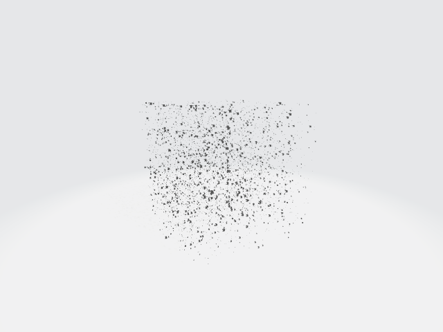
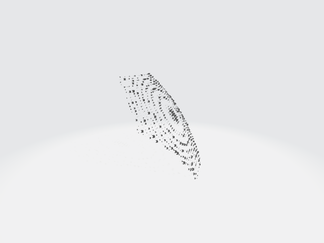
Recovery only up to level-sets in all three axes
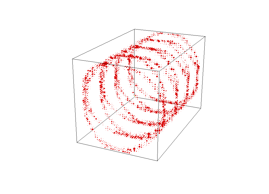
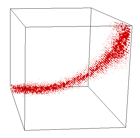
Recovery only up to level-sets in all three axes
Where is this coming from?
X = \begin{bmatrix} 1 & 1 & 1 \\ 1 & 1 & 1 \\ 1 & 1 & 0 \end{bmatrix}
t=\begin{bmatrix}1\\-1\\1\end{bmatrix}
t=\begin{bmatrix} 1\\ -1 \\ 1 \end{bmatrix} \to
Xt=\begin{bmatrix} 1\\ 1 \\ 0 \end{bmatrix} \to
X^2t=\begin{bmatrix} 2\\ 2 \\ 2 \end{bmatrix} \to
X^3 t=\begin{bmatrix} 4\\ 4 \\ 4 \end{bmatrix} \dashrightarrow
Stuff an infinite sequence
in a finite-dimensional space,
you get a dependence.
0=X^3t -2X^2 t=X^2(X-2I_3)t
So begins the story of annihilator polynomials and eigen values.
T =\begin{bmatrix} 1 & 0 & 3 \\ 4 & 5 & 6 \end{bmatrix}
X =\begin{bmatrix} 1 & 0 \\ 0 & 0 \end{bmatrix}
Y =\begin{bmatrix} 0 & 0 & 0 \\ 0 & 1 & 0 \\ 0 & 0 & 0
\end{bmatrix}.

(X^2-X)T\to x^2-x\\
T(Y^2-Y)\to y^2-y\\
XTY\to xy
An infinite lattice in finite-dimensional space makes even more dependencies.
(and the ideal these generate)
> M := Matrix(Rationals(), 2,3,[[1,0,2],[3,4,5]]);
> X := Matrix(Rationals(), 2,2,[[1,0],[0,0]] );
> Y := Matrix(Rationals(), 3,3,[[0,0,0],[0,1,0],[0,0,0]]);
> seq := [ < i, j, X^i * M * Y^j > : i in [0..2], j in [0..3]];
> U := Matrix( [s[3] : s in seq]);
        i   j   X^i * M * Y^j
        0   0   [ 1, 0, 2, 3, 4, 5 ]
        1   0   [ 1, 0, 2, 0, 0, 0 ]
        2   0   [ 1, 0, 2, 0, 0, 0 ]
        0   1   [ 0, 0, 0, 0, 4, 0 ]
        1   1   [ 0, 0, 0, 0, 0, 0 ]
        2   1   [ 0, 0, 0, 0, 0, 0 ]
        0   2   [ 0, 0, 0, 0, 4, 0 ]
        1   2   [ 0, 0, 0, 0, 0, 0 ]
        2   2   [ 0, 0, 0, 0, 0, 0 ]
        0   3   [ 0, 0, 0, 0, 4, 0 ]
        1   3   [ 0, 0, 0, 0, 0, 0 ]
        2   3   [ 0, 0, 0, 0, 0, 0 ]
In detail
Step out the bi-sequence
> E, T := EchelonForm( U );     // E = T*U
        0   0   [ 1, 0, 2, 3, 4, 5 ]    1
        1   0   [ 1, 0, 2, 0, 0, 0 ]    x
        0   1   [ 0, 0, 0, 0, 4, 0 ]    y
Choose pivots
Write null space rows as relations in pivots.
> A<x,y> := PolynomialRing( Rationals(), 2 );
> row2poly := func< k | &+[ T[k][1+i+3*j]*x^i*y^j :
     i in [0..2], j in [0..3] ] );
> polys := [ row2poly(k) : k in [(Rank(E)+1)..Nrows(E)] ];
        2   0   [ 1, 0, 2, 0, 0, 0 ]    x^2 - x
        1   1   [ 0, 0, 0, 0, 0, 0 ]    x*y
        2   1   [ 0, 0, 0, 0, 0, 0 ]    x^2*y
        0   2   [ 0, 0, 0, 0, 4, 0 ]    y^2 - y
        1   2   [ 0, 0, 0, 0, 0, 0 ]    x*y^2
        2   2   [ 0, 0, 0, 0, 0, 0 ]    x^2*y^2
        0   3   [ 0, 0, 0, 0, 4, 0 ]    y^3 - y
        1   3   [ 0, 0, 0, 0, 0, 0 ]    x*y^3
        2   3   [ 0, 0, 0, 0, 0, 0 ]    x^2*y^3
> ann := ideal< A | polys >;
> GroebnerBasis(ann);
    x^2 - x,
    x*y,
    y^2 - y
Take Groebner basis of relation polynomials
Groebner in bounded number of variables is in polynomial time (Bradt-Faugere-Salvy).
T =\begin{bmatrix} 1 & 0 & 3 \\ 4 & 5 & 6 \end{bmatrix}
I_2- X =\begin{bmatrix} 0 & 0 \\ 0 & 1 \end{bmatrix}
I_3- Y =\begin{bmatrix} 1 & 0 & 0 \\ 0 & 0 & 0 \\ 0 & 0 & 1
\end{bmatrix}.
(X^2-X)T\to x^2-x\\
T(Y^2-Y)\to y^2-y

Same tensor,
different operators,
can be different annihilators.
T =\begin{bmatrix} 1 & 2 & 3 \\ 4 & 5 & 6 \end{bmatrix}
X =\begin{bmatrix} 1 & 0 \\ 0 & 0 \end{bmatrix}
Y =\begin{bmatrix} 0 & 0 & 0 \\ 0 & 1 & 0 \\ 0 & 0 & 0
\end{bmatrix}.
(X^2-X)T\to x^2-x\\
T(Y^2-Y)\to y^2-y
Different tensor,
same operators,
can be different annihilators.

Data
T:\mathbb{M}_{a\times b}(K), X:\mathbb{M}_a(K), Y:\mathbb{M}_b(K)
Action by polynomials
a(x,y)\cdot T
= \left(\sum_{i,j:\mathbb{N}} \alpha_{ij} x^i y^j\right)\cdot T
= \sum_{i,j:\mathbb{N}}\alpha_{ij} X^iT Y^j.
Resulting annihilating ideal
\mathrm{ann}_{X,Y}(T) = \{
a(x,y):K[x,y]\mid
a(X,Y)T=0\}.
Could this be wild? Read below.
Annihilators
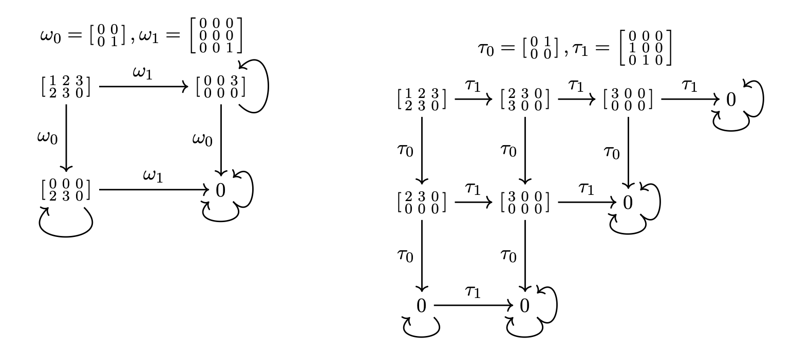


So given
- a tensor \(t\)
- a polynomial \(p(X)\)
- transverse operators \(\omega\)
\((\forall v)\,\langle t\mid p(\omega)\mid v\rangle=0\) just means \(p(X)\) is in the annihilator of this action.


Controlling Conenction
(First-Maglione-W.)
\(N(P,\Delta)=\{t\mid (\forall v)(\langle t\mid P(\Delta)|v\rangle=0)\}\) "closed" tensor space
\(I(S,\Delta)=\{p(X)\mid (\forall v)(\langle S\mid P(\Delta)|v\rangle=0)\}\) "closed" ideal
\(Z(S,P)=\{\omega\mid (\forall v)(\langle S\mid P(\omega)|v\rangle=0)\}\) "closed" scheme
Strategy
- tensors are the input data
- Polynomials are parameters we select
- Operator sets are what we want to explore our tensor
Summary of Trait Theorems (First-Maglione-W.)
- Linear traits correspond to derivations.
- Monomial traits correspond to singularities
- Binomial traits are only way to support groups.
For trinomial ideals, all geometries can arise so classification beyond this point is essentially impossible.
3 critically depends on Eisenbud-Sturmfels work on binomial ideals so it is restricted to vector spaces for now.
Derivations & Densors
Unintended Consequences
Since Whitney's 1938 paper, tensors have been grounded in associative algebras.
(A\subset \mathrm{End}(U)^{op}\times \mathrm{End}(V))\to U\otimes_A V
Derivations form natural Lie algebras.
[\delta,\delta'] = ([\delta'_0,\delta_0] , [\delta_1,\delta'_1],\ldots,[\delta_{\ell},\delta'_{\ell}] )\qquad\qquad\qquad \\
\qquad =(\delta'_0\delta_0-\delta_0\delta'_0,\delta_1\delta'_1-\delta'_1\delta_1,\ldots,\delta_{\ell}\delta'_{\ell}-\delta'_{\ell}\delta_{\ell})
If associative operators define tensor products but Lie operators are universal, who is right?
Tensor products are naturally over Lie algebras
Theorem (FMW). If
(\omega,\omega'\in Z(S,P)) \to\hspace{5cm}\\
\qquad(\omega_a\bullet \omega'_a = \alpha_{a}\omega_a\omega'_a+\beta_a \omega'_a\omega_a \in Z(S,P))
Then in all but at most 2 values of a
\langle (\alpha_a,\beta_a)\rangle = \langle (1,-1)\rangle \textnormal{ i.e. a Lie bracket}
In particular, to be an associative algebra we are limited to at most 2 coordinates. Whitney's definition is a fluke.
Module Sides no longer matter
- Whitney tensor product pairs a right with a left module, often forces technical op-ring actions.
- Lie algebras are skew commutative so modules are both left and right, no unnatural op-rings required.
V_1\otimes_{A_{10}} V_0 \textnormal{ vs. } V_0\otimes_{??} V_1
Associative Laws no longer
- Whitney tensor product is binary, so combining many modules consistantly by associativity laws isn't always possible - different coefficient rings.
(V_3\otimes_{A_{32}} V_2)\otimes_{A_{(32)1}} V_1 \textnormal{ vs. }
V_3\otimes_{??} (V_2\otimes_{??} V_1)
- Lie tensor products can be defined on arbitrary number of modules - no need for associative laws.
(\Delta\subset \prod_{a\in [\ell]} \mathfrak{gl}(V_a)) \to \hspace{2cm}\\
\qquad (| V_{\ell},\ldots,V_0 |)_{\Delta}=N(\Delta,D)
Missing opperators
- Whitney tensor product puts coefficient between modules only, cannot operate at a distance.
As valence grows we act on a linear number of spaces but have exponentially many possible actions left out.
V_3\otimes_{A_{32}} V_2\otimes_{A_{21}} V_1\textnormal{ vs. }
V_3\otimes_{A_{31}} V_1\otimes_{A_{12}} V_2
Lie tensor products act on all sides.
Densor
(| V_1,\ldots, V_n |)^{P}_{\Delta}=N(P,\Delta)
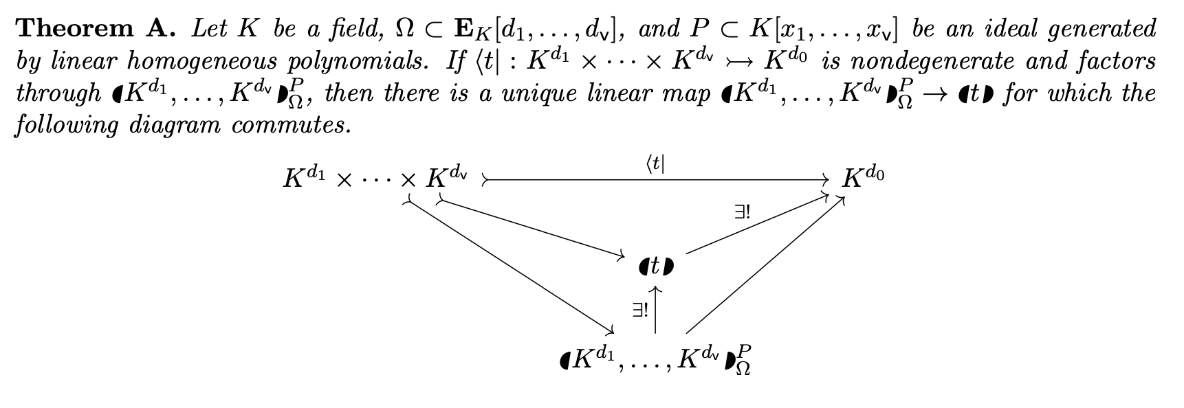
\((|t|):=N(x_1+\cdots+x_n,Z(t,x_1+\cdots+x_n))\)
Monomials, Singularities, & simplicial complexes

Shaded regions are 0.
Thm(FMW) Traits of operators that preserve a singularity have traits whose ideal is the Stanley-Reisner of complex.
(\langle t|U_A, V_{\bar{A}}\rangle =0)\quad \leftrightarrow \quad (X^e: I(t, \Omega_A), e=\chi_A)
Local Operators
(A <: [\ell]) \to ((a:A)\to (U_a<:V_a))\longrightarrow\\
\qquad\Omega_A =\prod_{a:A} U_a\oslash V_a\times \prod_{a:\bar{A}} V_a\oslash V_a
I.e. operators that on the indices A are restricted to the U's.
Claim. Singularity at U if, and only if, monomial trait on A.
Singularities come with traits that are in bijection with Stanley-Raisner rings, and so with simplicial complexes.
Binomials & Groups
Theorem (FMW). For fields. If for every S and P
(\omega,\omega'\in Z(S,P))\qquad
((\omega_a\omega'_a)^{\epsilon(a)}\mid a\in \{1,\ldots,\ell \})\in Z(S,P))
Q=(X^{e_1}-X^{f_1},\ldots, X^{e_m}-X^{f_m})
then \(\exists Q, Z(S,P)^{\times}=Z(S,Q)^{\times}\)
and \(\gcd\{e_1(a)+f_1(a),\ldots, e_m(a)+f_m(a)\}\in \{0,1\}\).
Converse holds if \(supp(e_1+\cdots +e_m)\cap supp(f_1+\cdots +f_m)=\emptyset\) even without conditions of a field. We speculate this is a necessary condition.
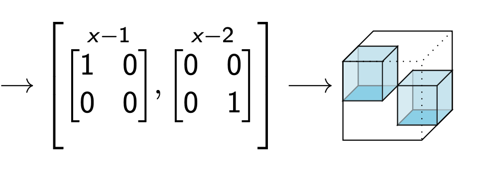
Back to decompositions
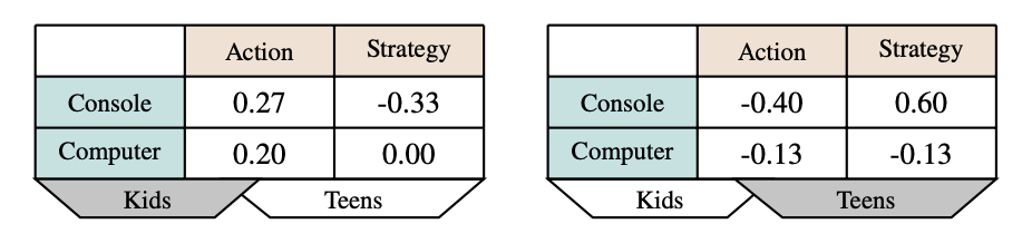
What are the markets?
Data table --> Multiplication table
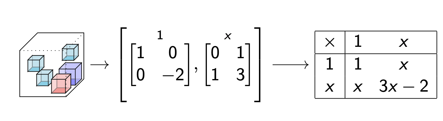
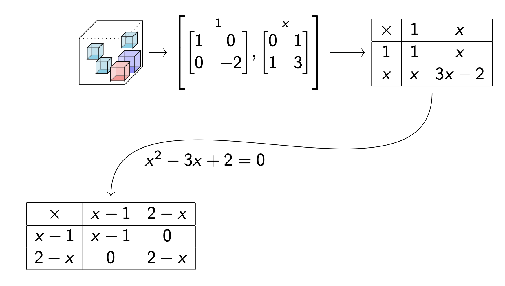
Use algebra to factor
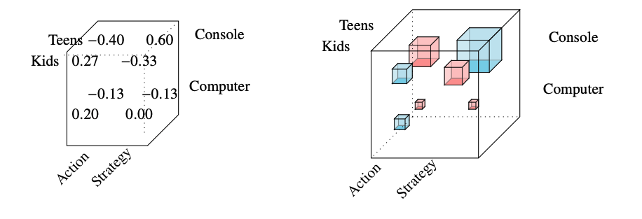
Forcing Good Algebra in Real Life
In real life the "multiplication" you get from a tensor is bonkers!
\begin{array}{c|ccc|} * & f_1 & f_2 & f_3 \\
\hline e_1 & 0.2g_1+0.9g_2-0.4g_3 & 0.2g_1+0.9g_2-0.4g_3 & -1.0g_1+0.4g_2-0.1g_3\\
e_1 & -9.1g_1+8.9g_2+0.7g_3 & -2.0g_1+0.1g_2-0.1g_3 & 0.0g_1+1.8g_2-0.4g_3 \\
\hline & & \end{array}
\[*:\mathbb{R}^2\times \mathbb{R}^3\to \mathbb{R}^3\]
Get to 100's 1000's of dimensions and you have no chance to know this algebra.
Study a function by its changes, i.e. derivatives.
Study multiplication by derivatives:
\[\partial (f·g ) = (\partial f )·g + f·(\partial g ).\]
In our context discretized. I.e. ∂ is a matrix D.
\[D(f ∗g ) = D(f ) ∗g + f ∗D(g )\]
And it is heterogeneous, so many D's
\[D_0(f*g) = D_1(f)*g + f * D_2(g).\]
For general tensors \[\langle t| : U_{1}\times \cdots \times U_{\ell}\to U_0\] there are many generalizations.
E.g.
\begin{aligned}
D_0\langle t|u_1,u_2,u_3\rangle & = \langle t|D_1u_1,u_2,u_3\rangle+ \langle t|u_1,D_2u_2,u_3\rangle\\
D_0\langle t|u_1,u_2,u_3\rangle&= \langle t|D_1u_1,u_2,u_3\rangle+ \langle t|u_1,u_2,D_3 u_3\rangle \\
D_0\langle t|u_1,u_2,u_3\rangle&= \langle t|u_1,D_2u_2,u_3\rangle+ \langle t|u_1,u_2,D_3u_3\rangle
\end{aligned}
Or \[ D_0\langle t |u_1,u_2, u_3\rangle = \langle t| D_1 u_1, u_2,u_3\rangle + \langle t| u_1, D_2 u_2, u_3\rangle + \langle t|u_1, u_2, D_3 u_3\rangle.\]
For general tensors \[\langle t| : U_{1}\times \cdots \times U_{\ell}\to U_0\]
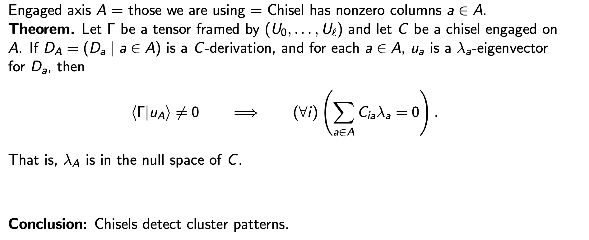
Choose a "chisel" (dleto) an augmented matrix C.
Write \[\langle \Gamma | C(D)|u\rangle =0\] to mean:
means chisel
\begin{array}{|ccc|c|} \hline 7 & -9 & 0 & 2\\ 1 & 1 & 1 & 1 \\ 0 & 1 & 1 & 1 \\ \hline \end{array}
And it's solutions are a Lie algebra
The main fact
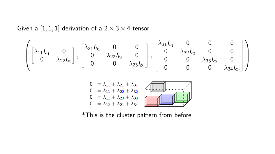
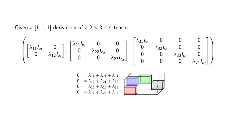
Summary
Cluster Patterns Theory
By James Wilson
Cluster Patterns Theory
A visual tour of how volume leads to tensors.


