MAgPIE 4.0
Open Source land-use modeling framework

Jan Philipp Dietrich
dixyzetrich@pik-xyzpotsdam.de


What is ?

Basics
Model of Agricultural Production and its Impact on the Environment
MAgPIE
cost minimization of consecutive time slices with a length of 5-20 years until 2100
dynamic recursive optimization
global | 5-20 world regions | 50-2000 spatial cluster
3 spatial layers
bringing together biophysical (plant growth, carbon, nutrients, water) and economic (costs, prices, demand, policies) aspects
balance biophysical and economic side

Basics
World Regions

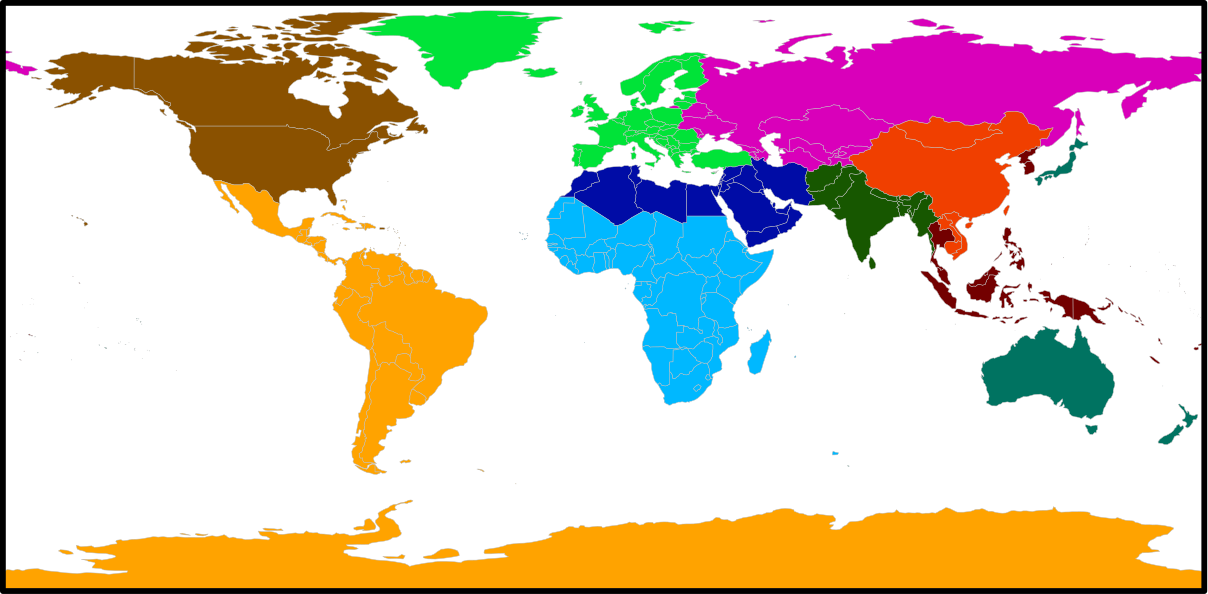

ISO countries
MAgPIE default 10 regions
Big Player & Fossil energy
Spatial
Cluster
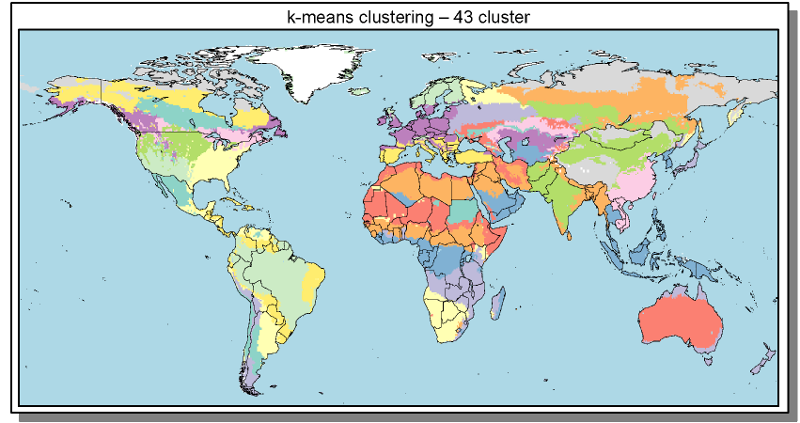
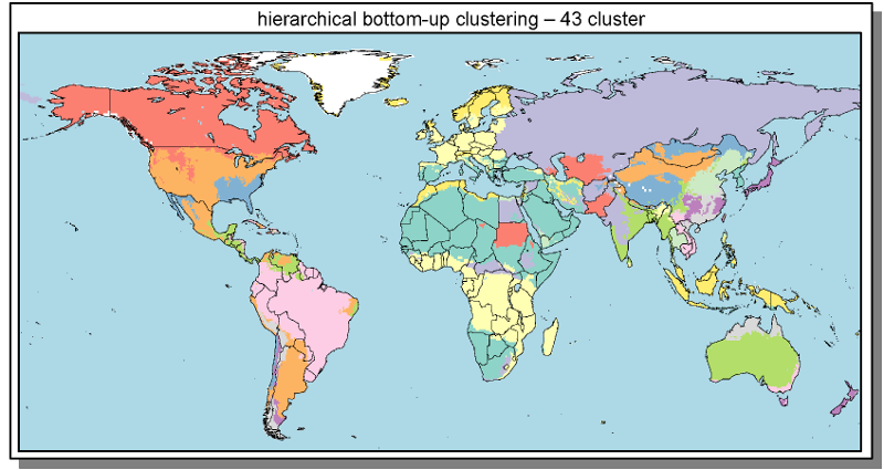
- Cluster build from 0.5° grid cells
- Clustering based on similarity of spatial explicit model inputs
- Outputs interpolated to 0.5° for visualization & analysis
Model Outputs


REMIND-MAgPIE Integrated Assessment Model
Model cascade
PIAM - Potsdam Integrated Assessment Modelling Framework
code

Requirements
-
GAMS (non-free)|gams.com
including license for solver CONOPT and CPLEX - R (free) | r-project.org
-
R packages (free)
README.md in MAgPIE lists all packages currently required - GIT (free) | git-scm.com
Recommendations
-
Modern text editor
e.g. Atom | atom.io -
Rstudio | rstudio.com
R editor -
PIK-CRAN | rse.pik-potsdam.de
PIK R package repository - GitHub account | github.com
First steps / get the code
- Fork MAgPIE repository @ github.com/magpiemodel/magpie
make a copy of the repository in GitHub
- Clone forked repository
download the copy to your machine
- Follow instructions in README.md
- Run the model
Code Structure #1
GAMS Model Core
- model equations
- modules
- model simulation
R Pre- & Postprocessing Layer
- model configuration
- data download
- run management
- run compilation
- output processing
- visualization
- Model development in GAMS
- Model application in R
- R used to boost GAMS capabilities
Code Structure #2
GAMS Model Core
- core
- module 1
- realization A
- realization B
- module 2
- realization A
- realization B
- realization C
- module 1
...
- split a big system into many small components
- flexibility to switch between different implementations


GAMS Modules
Code Structure #3
Naming conventions to..
- improve readability
- emulate local environments in GAMS
q13_cost_tc(i2) ..
  v13_cost_tc(i2) =e= sum(ct, i13_land(i2) * i13_tc_factor(ct,i2)
                     * vm_tau(i2)**i13_tc_exponent(ct,i2)
                     * (1+pm_interest(i2))**15);
1st Prefix q - eQuation v - Variable i - Input parameter p - Parameter
...
2nd Prefix
?m - module interface
?00 - module-internal
(2-digit module code)
more details:
Repository Structure
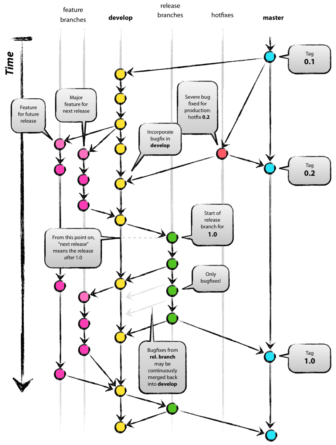
- official releases in master branch
- most recent version in develop
- release candidates in release branch
- development in feature branches (f_<name>)
Configuration | default.cfg
# |  (C) 2008-2018 Potsdam Institute for Climate Impact Research (PIK),
# |  authors, and contributors see AUTHORS file
# |  This file is part of MAgPIE and licensed under GNU AGPL Version 3
# |  or later. See LICENSE file or go to http://www.gnu.org/licenses/
# |  Contact: magpie@pik-potsdam.de

##################
#### SETTINGS ####
##################

cfg <- list()

#### Main settings ####

# short description of the actual run
cfg$title <- "default"

# path to the submodel to be used relative to main model folder
cfg$model <- "main.gms"   #def = "main.gms"

#### input settings ####

# which input data sets should be used?
cfg$input <- c("isimip_rcp-IPSL_CM5A_LR-rcp2p6-noco2_rev29_h200_8a828c6ed5004e77d1ba2025e8ea2261.tgz",
               "rev3.15_8a828c6ed5004e77d1ba2025e8ea2261_magpie.tgz",
               "rev3.15_8a828c6ed5004e77d1ba2025e8ea2261_validation.tgz",
               "additional_data_rev3.29.tgz",
               "npi_ndc_base_SSP2_mixed.tgz")

#a list of repositories (please pay attention to the list format!) in which the
#files should be searched for. Files will be searched in all repositories until
#found, always starting with the first repository in the list. The argument must
#have the format of a named list with the url of the repository as name and a
#corresponding list of options such as username or password to access the
#repository as value. If no options are required the value has to be NULL. (e.g.
#list("ftp://my_pw_protected_server.de/data"=list(user="me",password=12345),
#     "http://free_server.de/dat"=NULL))
#Please add system or user specific repositories (such as repos with limited
#access for) through the R option "magpie_repos". Through the append command
#below it will get merged into cfg$repositories

cfg$repositories <- append(list("https://rse.pik-potsdam.de/data/magpie/public"=NULL),
                           getOption("magpie_repos"))


# Should input data be downloaded from source even if cfg$input did not change?
cfg$force_download <- FALSE

# Settings for the yield calibration
# * (TRUE): Yield calibration will be performed
# * (ifneeded): Yield calibration will only be executed if input data is
# *             downloaded from repository
# * (FALSE): Yield calibration will not be performed
cfg$recalibrate <- "ifneeded"     # def = ifneeded
# Up to which accuracy shall be recalibrated?
cfg$calib_accuracy <- 0.1         # def = 0.1
# What is the maximum number of iterations if the precision goal is not reached?
cfg$calib_maxiter <- 20           # def = 20
# factor determining how much the new calibration factor influences the result
# (0-1)
cfg$damping_factor <- 0.98        # def= 0.98
# switch on/of calibration of cropland (pasture will be left untouched)
cfg$calib_cropland <- TRUE         # def= TRUE


# Settings for NPI/NDC recalculation
# * (TRUE): NPI/NDC recalculation will be performed
# * (ifneeded): NPI/NDC recalculation will only be executed if current input files
# *             are zero and policy switches (p32_aff_pol, p35_ad_pol, p35_emis_pol)
# *             are set to "npi" or "ndc". If policy switches are set to "none"
# *             (default) NPI/NDC recalculation will not be performed
# * (FALSE): NPI/NDC recalculation will not be performed
cfg$recalc_npi_ndc <- TRUE    # def = ifneeded
# * should the new base run be calculated?
cfg$recalc_base_run <- FALSE
# * which national or subnational mappinng should be used
cfg$policyregions <- "iso"           # def = "iso"

#### magpie.gms settings ####
cfg$gms <- list()

# Set number of time steps (1-16) or type "less_TS" for remind time steps
cfg$gms$c_timesteps <- 10

# use of gdx files
cfg$gms$s_use_gdx <- 2  # def = 2
#*                   0:  gdx will not be loaded
#*                   1:  gdx is loaded in the first time step
#*                   2:  gdx is loaded in all time steps

# **----------------------------------------------------------------------------
# ***                           MODULES
# ***---------------------------------------------------------------------------

# ***---------------------    09_drivers   ----------------------------------------
# * (aug17): default drivers
cfg$gms$drivers <- "aug17"          # def = aug17
cfg$gms$c09_pop_scenario  <- "SSP2"    # def = SSP2
cfg$gms$c09_gdp_scenario  <- "SSP2"    # def = SSP2
# *   options:   SSP: "SSP1", "SSP2", "SSP3", "SSP4", "SSP5"
# *             SRES: "A1", "A2", "B1", "B2"

# ***---------------------    10_land   ----------------------------------------
# * (feb15): default land realization
cfg$gms$land <- "feb15"          # def = feb15


# ***---------------------    11_costs   ------ --------------------------------
# * (default): default cost realization
cfg$gms$costs <- "default"          # def = default

# ***---------------------    12_interest_rate ---------------------------------
# * (glo_jan16): global interest rates - annuity calculated with macro m_annuity
# * (reg_feb18): regional interest rates, dependent on development state

cfg$gms$interest_rate <- "reg_feb18"          # def = reg_feb18

# * interest rate scenario: low, medium, high or mixed
cfg$gms$c12_interest_rate <- "medium"          # def = "medium"

# * investment time horizon (years)
cfg$gms$sm_invest_horizon <- 30                # def = 30

# ***---------------------    13_tc    -----------------------------------------
# * (endo_JUN16): endogenous technological change with full cost accounting
cfg$gms$tc <- "endo_JUN16"              # def = endo_JUN16

# * tc cost scenario: low, medium or high
cfg$gms$c13_tccost <- "medium"

# ***---------------------    14_yield    --------------------------------------
# * (biocorrect): yield calculations with correction for bioenergy crops
# * (staticpasture): no yield increases for pasture
# * (dynamic_apr18): dynamic pasture yield calculation
cfg$gms$yields <- "biocorrect"          # def = biocorrect

# * yield scenario
# *   options:   cc  (climate change)
# *             nocc (no climate change)
cfg$gms$c14_yields_scenario  <- "nocc"   # def = "nocc"

# * switch determing the effectivity of translating crop tc into pasture yield
# * increase. Value has to be in the range of 0 (no pasture yield growth)
# * and 1 (pasture yields increase linearily with tau)
cfg$gms$s14_yld_past_switch <- 0.25           # def = 0.25

# ***---------------------    15_food    ---------------------------------------
# * (anthropometrics_jan18): estimates food using scenario dependent regression
# *                          and demography drivers
cfg$gms$food <- "anthropometrics_jan18"            # def = anthropometrics_jan18

# * maximal number of iterations between food and magpie model before
# * simulation proceeds to next time step
cfg$gms$s15_maxiter <- 5                   # def = 5

# * convergence criteria: maximal allowed country-wise deviation in calculated
# *                       real income between iterations
cfg$gms$s15_convergence <- 0.05            # def = 0.05

# * switch between exogenous and endogenous food demand
# *  options: 0 (exogenous food demand) and 1 (endogenous food demand)
cfg$gms$s15_elastic_demand <- 1            # def =1

# * food scenario
# *   options:   SSP: "SSP1", "SSP2", "SSP3", "SSP4", "SSP5"
# *             SRES: "A1", "A2", "B1", "B2"
# *            OTHER: "PB" (planetary boundaries)
cfg$gms$c15_food_scenario <- "SSP2"        # def = SSP2

# * ruminant meat share scenario
# *   options:   constant, halving2050, mixed
cfg$gms$c15_rumscen <- "mixed"             # def = mixed

# ***---------------------    16_demand    -------------------------------------
# * (sector_may15): default for flexible regions
cfg$gms$demand <- "sector_may15"                # def = sector_may15

# ***---------------------    17_production    ---------------------------------
# * (flexreg_apr16): default production aggregation
cfg$gms$production <- "flexreg_apr16"          # def = flexreg_apr16

# ***---------------------    18_residues    -----------------------------------
# * (flexreg_apr16): detailed residue calculations
# * (off): off
cfg$gms$residues <- "flexreg_apr16"            # def = flexreg_apr16

# ***---------------------    20_processing    ---------------------------------
# * (coupleproducts_feb17): processing with couple products
# * (off): off
cfg$gms$processing <- "coupleproducts_feb17"        # def = coupleproducts_feb17

# ***---------------------    21_trade    --------------------------------------
# * (free_apr16):       free trade without restrictions
# * (off):              no trade at all
# * (selfsuff_flexreg): self-sufficiency based trade
# * (selfsuff_flexreg_cost): self-sufficiency based trade with trade costs related to exports
cfg$gms$trade <- "selfsuff_flexreg_cost"             # def = selfsuff_flexreg_cost

# * trade balance reduction scenario
# * (regionalized): regionalized trade balance reduction
# * (globalized):   globalized trade balance reduction
# * (fragmented):   fragmented trade balance reduction
cfg$gms$c21_trade_liberalization  <- "regionalized"       # def = regionalized

# * whether trade tariff should be considered
# * (0) without trade tariff
# * (1) with  trade tariff
cfg$gms$s21_trade_tariff <- 0               # def =0

# ***---------------------    30_crop    ---------------------------------------
# * (endo_jun13): dynamic cropland
cfg$gms$crop    <- "endo_jun13"               # def = endo_jun13

# ***---------------------    31_past    ---------------------------------------
# * (static):     static pasture
# * (endo_jun13): dynamic pasture
cfg$gms$past <- "endo_jun13"               # def = endo_jun13

# * Factor requirements (US$04 per ton DM)
cfg$gms$s31_fac_req_past  <- 1             # def = 1

# ***---------------------    32_forestry    -----------------------------------
# * (static_sep16) :     static forestry sector
# * (affore_vegc_dec16): static forestry sector + afforestation
cfg$gms$forestry  <- "affore_vegc_dec16"              # def = affore_vegc_dec16

# Afforestation policy
# * ("none"): no prescribed afforestation
# * ("npi"): prescribed afforestation based on NPI policies
# * ("ndc"): prescribed afforestation based on NPI+NDC policies
cfg$gms$c32_aff_policy <- "npi"              # def = "none"

# maximum total global afforestation in Mha (Inf = no constraint)
cfg$gms$s32_max_aff_area <- Inf              # def = Inf

# Switch to determine whether afforestation should be limited to
# certain latitudinal zones
# * ("unrestricted"): No regions excluded
# * ("noboreal"): Exclude boreal regions > 50deg N
# * ("onlytropical"): Afforestation only in tropical areas 20deg S-20deg N
cfg$gms$c32_aff_mask <- "noboreal"            # def = "noboreal"

# ***---------------------    34_urban   ---------------------------------------
# * (static): static urban
cfg$gms$urban   <- "static"                # def = static

# ***---------------------    35_natveg    --------------------------------------
# * 35_natveg includes primforest, secdforest and other land
# * (static):               static natveg land
# * (dynamic_mai17): 		dynamic natveg land
cfg$gms$natveg  <- "dynamic_mai17"           # def = dynamic_mai17

# * protected areas (primforest,secdforest,other land)
# * (WDPA) WDPA IUCN catI+II
# * (BH) Biodiversity Hotspots + WDPA
# * (FF) Frontier Forests + WDPA
# * (CPD) Centres of Plant Diversity + WDPA
# * (LW) last of the wild + WDPA
# * (none) no protection
# * (full) full protection
cfg$gms$c35_protect_scenario <- "WDPA"			# def = WDPA

# Avoided Deforestation policy
# * ("none"): no avoided deforestation
# * ("npi"): avoided deforestation based on NPI policies
# * ("ndc"): avoided deforestation based on NPI+NDC policies
cfg$gms$c35_ad_policy <- "npi"              # def = "none"

# Land-use change emission reduction policy (emissions from primforest and secdforest)
# * ("none"): no emission reduction policy
# * ("npi"): emission reduction policy based on NPI policies
# * ("ndc"): emission reduction policy based on NPI+NDC policies
cfg$gms$c35_emis_policy <- "npi"              # def = "none"

# ***---------------------    38_factor_costs    -------------------------------
# * (fixed_per_ton_nov16): factor costs fixed per ton
# * (mixed_feb17):         reimplementation of MAgPIE 3.0 default
cfg$gms$factor_costs <- "mixed_feb17"        # tentative default = mixed_feb17

# ***---------------------    39_landconversion    -----------------------------
# * (gdp_scaled_jun13): gdp based land conversion costs (new parametrization)
# * (gdp_vegc_mar18): land clearing costs based on GDP and vegetation carbon density.
# *                   Land establishment costs based on GDP
cfg$gms$landconversion <- "gdp_vegc_mar18"     # def = gdp_vegc_mar18

# * land conversion cost scenario (works only with gdp_vegc_mar18)
# *   options:  low, medium, high
cfg$gms$c39_cost_scenario  <- "high"   # def = "high"

# ***---------------------    40_transport    ----------------------------------
# * (off):        no transport costs
# * (gtap_nov12): transport costs applied to crops and ruminant livestock
# *               products calibrated based on magpie-output (dynamic pasture)
# *               to match GTAP data
cfg$gms$transport <- "gtap_nov12"                   # def = gtap_nov12

# ***---------------------    41_area_equipped_for_irrigation    ---------------
# * (static):     no expansion
# * (endo_APR13): endogenous, cost driven expansion
cfg$gms$area_equipped_for_irrigation <- "endo_apr13"   # def = endo_APR13

# ***---------------------    42_water_demand   --------------------------------
# * (agr_sector_aug13): fixed fraction of water available is reserved
# *                     for other uses
# * (all_sectors_aug13): industrial, eletricity and domestic demand are
# *                     retrieved from WATERGAP data.
cfg$gms$water_demand<- "agr_sector_aug13"            # def = agr_sector_aug13

# * water demand scenario
# *   options:   cc  (climate change)
# *             nocc (no climate change)
cfg$gms$c42_watdem_scenario  <- "nocc"   # def = "nocc"

# * Choice of fraction of available water that is not
# * available for agriculture (only affects agr_sector_aug13 realization)
cfg$gms$s42_reserved_fraction <- 0.5         # def = 0.5

# * Scenario for non agricultural water demand from WATERGAP
# * (only affects all_sector_aug13 realization)
# * (1): SSP2
# * (2): A2
# * (3): B1
cfg$gms$s42_watdem_nonagr_scenario <- 1      # def = 1

# * Switch to determine the irrigation efficiency scenario
# * (1): global static value
# * (2): regional static values from gdp regression
# * (3): gdp driven increase
cfg$gms$s42_irrig_eff_scenario <- 1           # def = 1

# * Environmental flow protection policy
# * (off):   no EFP policy
# * (on):    global EFP policy starting in 2015
# * (mixed): EFP policy starting in 2015 only in hic regions
cfg$gms$c42_env_flow_policy <- "off"             # def = "off"

# * Environmental flow protection scenario
# * (0): do not consider environmental flows.
# *      s42_env_flow_base_fraction and
# *      s42_env_flow_fraction have no effect.
# * (1): Reserve a certain fraction of available water
# *      specified by s42_env_flow_fraction for
# *      environmental flows
# * (2): Each grid cell receives its own value for
# *      environmental flow protection based on LPJ
# *      results and a calculation algorithm by Smakhtin 2004.
# *      s42_env_flow_fraction has no effect.
cfg$gms$s42_env_flow_scenario <- 2             # def = 2

# * Fraction of available water that is reserved for the environment
# * in case of a protection policy
# * In which regions and timesteps a protection policy is in place is determined
# * in the file EFR_protection_policy.csv in the input folder
# * of the 42_water_demand module
cfg$gms$s42_env_flow_fraction <- 0.2           # def = 0.2

# * Fraction of available water that is reserved for the environment in case of
# * missing protection policy
cfg$gms$s42_env_flow_base_fraction <- 0.05      # def = 0.05

# ***---------------------    43_water_availability   --------------------------
# * (total_water_aug13): surface and ground water resources available
cfg$gms$water_availability <- "total_water_aug13"    # def = total_water_aug13

# * water availability scenario
# *   options:   cc  (climate change)
# *             nocc (no climate change)
cfg$gms$c43_watavail_scenario  <- "nocc"   # def = "nocc"

# ***-------------------------    45_climate   ---------------------------------
# * (static): static koeppengeiger climate classification data
cfg$gms$climate <- "static"    # def = static

# ***-------------------------    50_nr_soil_budget   --------------------------
# * (off):          off
# * (exoeff_aug16): exogenous nr efficiency
cfg$gms$nr_soil_budget <- "exoeff_aug16"    # def = exoeff_aug16

# * options: neff55_55_starty1990,neff60_60_starty1990,neff65_70_starty1990,
# *          neff65_70_starty2010,neff60_60_starty2010,neff55_60_starty2010,
# *          neff70_75_starty2010,neff75_80_starty2010,neff80_85_starty2010
cfg$gms$c50_scen_neff <- "neff60_60_starty2010"   # def = neff60_60_starty2010

# ***---------------------    51_nitrogen   ------------------------------------
# * (ipcc2006_sep16): IPCC based nitrogen implementation
# * (off):            no nitrogen calculations
cfg$gms$nitrogen    <- "ipcc2006_sep16"                 # def = ipcc2006_sep16

# ***---------------------    52_carbon   --------------------------------------
# * (normal_sep16): regrowth of carbon stocks starts from 0 in vegc and litc pools,
# * and from mean of cropland and pasture in soilc pool
# * (normal_dec17): regrowth of carbon stocks in all c pools starts from pasture levels
# * (off):          carbon calculations deactivated
cfg$gms$carbon <- "normal_dec17"                       # def = normal_dec17

# * carbon scenario
# *   options:   cc  (climate change)
# *             nocc (no climate change)
cfg$gms$c52_carbon_scenario  <- "nocc"   # def = "nocc"

# ***---------------------    53_methane   -------------------------------------
# * (ipcc2006_flexreg_apr16): IPCC 1996 methodology
# * (off):                    methane calculations deactivated
cfg$gms$methane  <- "ipcc2006_flexreg_apr16"    # def = ipcc2006_flexreg_apr16

# ***---------------------    54_phosphorus   ----------------------------------
# * (off): calculations deactivated
cfg$gms$phosphorus  <- "off"                     # def = off

# ***---------------------    55_awms   ---------------------------------------
# * (ipcc2006_aug16): animal waste management systems
# *                   (based on IPCC 2006 Guidelines)
# * (off):            deactivated animal waste management
cfg$gms$awms  <- "ipcc2006_aug16"                     # def = ipcc2006_aug16

# ***---------------------    56_ghg_policy   ----------------------------------
# * (price_sep16): GHG emission pricing - same annuity as used in other modules
cfg$gms$ghg_policy  <- "price_sep16"                     # def = price_sep16

# * pollutant price scenario
cfg$gms$c56_pollutant_prices <- "SSP2-Ref-SPA0"         # def = "SSP2-Ref-SPA0"
# *   options:  SSP1-Ref-SPA0, SSP2-Ref-SPA0, SSP5-Ref-SPA0,
# *             SSP1-26-SPA0, SSP1-37-SPA0, SSP1-45-SPA0,
# *             SSP2-26-SPA0, SSP2-37-SPA0, SSP2-45-SPA0, SSP2-60-SPA0,
# *             SSP5-26-SPA0, SSP5-37-SPA0, SSP5-45-SPA0, SSP5-60-SPA0,
# *             SSP1-26-SPA1, SSP1-37-SPA1, SSP1-45-SPA1,
# *             SSP2-26-SPA2, SSP2-37-SPA2, SSP2-45-SPA2, SSP2-60-SPA2,
# *             SSP5-26-SPA5, SSP5-37-SPA5, SSP5-45-SPA5, SSP5-60-SPA5,
# *             coupling

# * emission policies
# * options: none, all, ssp
# * ssp: CO2 emis from LUC in natveg; all CH4 and N2O emissions
cfg$gms$c56_emis_policy <- "ssp" 		# def = ssp

# * Treatment of negative costs originating from negative co2 emissions
# * reward negative co2 emissions (-Inf) or not (0)
# * s56_reward_neg_emis is applied on emission policy chosen in c56_emis_policy
# * In case of carbon pricing s56_reward_neg_emis = -Inf results in increase of other land
# * For runs with afforestation s56_reward_neg_emis should be 0 (default setting)
cfg$gms$s56_reward_neg_emis <- 0			# def = 0

# * economic incentive for afforestation (only effective if forestry=affore_vegc_dec16)
# * options: none, all, all50, vegc50, vegc33, vegc25
# * none: no carbon price applied on forestry carbon pools
# * all: full carbon price; all carbon pools
# * all50: 50% of carbon price; all carbon pools
# * vegc50: 50% of carbon price; only vegetation carbon pool
# * vegc33: 33% of carbon price; only vegetation carbon pool
# * vegc25: 25% of carbon price; only vegetation carbon pool
cfg$gms$c56_aff_policy <- "vegc33"		# def = vegc33

# ***---------------------    57_maccs   ---------------------------------------
# * (on_sep16):  maccs for non-CO2 emission mitigation activated
# * (off_jul16): maccs for non-CO2 emission mitigation deactivated
cfg$gms$maccs  <- "on_sep16"                     # def = on_sep16

# ***---------------------    58_carbon_removal   ------------------------------
# * (off_sep16): deactivated
cfg$gms$carbon_removal <- "off_sep16"                  # def = off_sep16

# ***-------------------------    59_som   -------------------------------------
# * (off): off
# * (cellpool_aug16): soil organic matter pool on cellular level
cfg$gms$som <- "off"    # def = off

# ***---------------------    60_bioenergy   -----------------------------------
# * (standard_flexreg_may17): fixed 1st generation demand based on Lotze Campen (2014),
# *                           scenario-depending 2nd gen demand which can be
# *                           either fullfilled by begr or betr
cfg$gms$bioenergy <- "standard_flexreg_may17"     # def = standard_flexreg_may17

# * 1st generation bioenergy demand scenarios based on Lotze Campen (2014)
# * (phaseout2020): increase until 2020, followed by phaseout until 2050
# * (const2020): increase until 2020, constant thereafter
# * (const2030): increase until 2030, constant thereafter
cfg$gms$c60_1stgen_biodem <- "const2020"               # def = const2020

# * 2nd generation bioenergy demand scenarios for standard realization
# *   options:  SSP1-Ref-SPA0, SSP2-Ref-SPA0, SSP5-Ref-SPA0,
# *             SSP1-26-SPA0, SSP1-37-SPA0, SSP1-45-SPA0,
# *             SSP2-26-SPA0, SSP2-37-SPA0, SSP2-45-SPA0, SSP2-60-SPA0,
# *             SSP5-26-SPA0, SSP5-37-SPA0, SSP5-45-SPA0, SSP5-60-SPA0,
# *             SSP1-26-SPA1, SSP1-37-SPA1, SSP1-45-SPA1,
# *             SSP2-26-SPA2, SSP2-37-SPA2, SSP2-45-SPA2, SSP2-60-SPA2,
# *             SSP5-26-SPA5, SSP5-37-SPA5, SSP5-45-SPA5, SSP5-60-SPA5,
# *             coupling
cfg$gms$c60_2ndgen_biodem <- "SSP2-Ref-SPA0"     # def = SSP2-Ref-SPA0

# * bioenergy demand level
# * (1): regional
# * (0): global
cfg$gms$c60_biodem_level <- 1                     # def = 1

# ***---------------------    62_material   ------------------------------------
# * (exo_flexreg_apr16): default
cfg$gms$material <- "exo_flexreg_apr16"

cfg$gms$c62_material_scenario <- "SSP2"

# ***---------------------    70_livestock   -----------------------------------
# * (fbask_jan16): default feed basket realization
cfg$gms$livestock <- "fbask_jan16"                  # def = fbask_jan16

# * feed scenario
# *   options:    ssp1, ssp2, ssp3, ssp4, ssp5, constant
cfg$gms$c70_feed_scen <- "ssp2"                     # def = ssp2

# ***-------------------    80_optimization ------------------------------------
# * (nlp_apr17):    solve procedure solving the whole, nonlinear problem
# *                 at once
# * (lp_nlp_apr17): alternative approach in which the nonlinear terms are
# *                 fixed first so that the linear problem can be solved
# *                 before the full problem is solved
cfg$gms$optimization <- "lp_nlp_apr17"              # def = lp_nlp_apr17

# maximal number of solve iterations
cfg$gms$s80_maxiter <- 30

# * (conopt3):         conopt3
# * (conopt4):         conopt4
# * (conopt4+cplex):   conopt4 followed by cplex with landdiff optimization
# * (conopt4+conopt3): conopt4 followed by conopt3
cfg$gms$c80_nlp_solver <- "conopt4+conopt3"              # def = conopt4

# * 1: using optfile for specified solver settings
# * 0: default settings (optfile will be ignored)
cfg$gms$s80_optfile <- 1


#*******************************END MODULE SETUP********************************

#### Other settings (e.g. clustering, gdx files, ...): ####

# Decide whether the runs should be run sequentially (TRUE),
# or in parallel (FALSE)
# NA means that this decision is taken automatically
# (typically on cluster = FALSE and locally = TRUE)
cfg$sequential <- NA

# How should log information be treated?
# (0:no output, 2:write to full.log 3:show in console)
cfg$logoption <- 2

# Should output.R generate output?
# List of output scripts that should be used
# Available scripts can be found in scripts/output/
cfg$output <- c("rds_report",
                "validation",
                "interpolation",
                "DiffPlot_CropReshuffle",
                "LU_DiffPlots",
                "LandusePlots")

# Set the format for the results folder
# :date: is a placeholder for the current time stamp (e.g. "results:date:")
# :title: is a placeholder for the current run title (cfg$title)
cfg$results_folder <- "output/:title::date:"

# Which files should be copied into the output folder?
cfg$files2export <- list()
# Files that should be copied before MAgPIE is started
cfg$files2export$start <- c("input/info.txt",
                            "modules/10_land/input/avl_land.cs3",
                            "input/spatial_header.rda",
                            "scripts/run_submit/submit.R",
                            "scripts/run_submit/submit.sh",
                            ".Rprofile",
                            "input/*.spam",
                            "input/validation.mif")
# Files that should be copied after the MAgPIE run is finished
cfg$files2export$end <- NULL

# Folder run statistics should be submitted to
cfg$runstatistics <- "/p/projects/rd3mod/models/statistics/magpie"

# name of the overall model (just used for reporting purposes)
# should usually not be changed
cfg$model_name <- "MAgPIE"

# model version of the overall model (use extension "-rc" for release candidate
# and "-dev" for developer version)
cfg$model_version <- "4.0-rc"

# Should the model run in developer mode? This will loosen some restrictions,
# such as temporary toleration of coding etiquette violations
# Please make sure to set it to FALSE for production runs!
cfg$developer_mode <- FALSE

# Should the model run in debug mode?
# Download script will copy files from input to destination folder instead of
# moving it allowing to check whether something in the move/copy process goes
# wrong
cfg$debug <- FALSE

################################################################################
Start & Output scripts
Rscript start.R

Choose start script:
1: default
2: check code
3: download data only
4: cemics2
5: emulator
6: sim4nexus
7: sustag
8: testruns
Number: 1

Choose submission type:
1: Direct execution
2: Background execution
3: Debug mode
Number:
# |  (C) 2008-2018 Potsdam Institute for Climate Impact Research (PIK),
# |  authors, and contributors see AUTHORS file
# |  This file is part of MAgPIE and licensed under GNU AGPL Version 3
# |  or later. See LICENSE file or go to http://www.gnu.org/licenses/
# |  Contact: magpie@pik-potsdam.de


######################################
#### Script to start a MAgPIE run ####
######################################

# Load start_run(cfg) function which is needed to start MAgPIE runs
source("scripts/start_functions.R")

#start MAgPIE run
start_run(cfg="default.cfg")
Applications

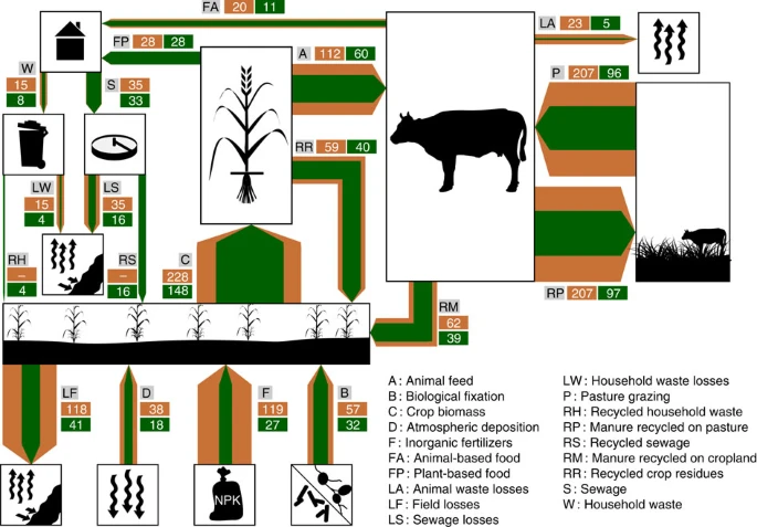
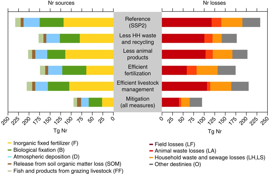


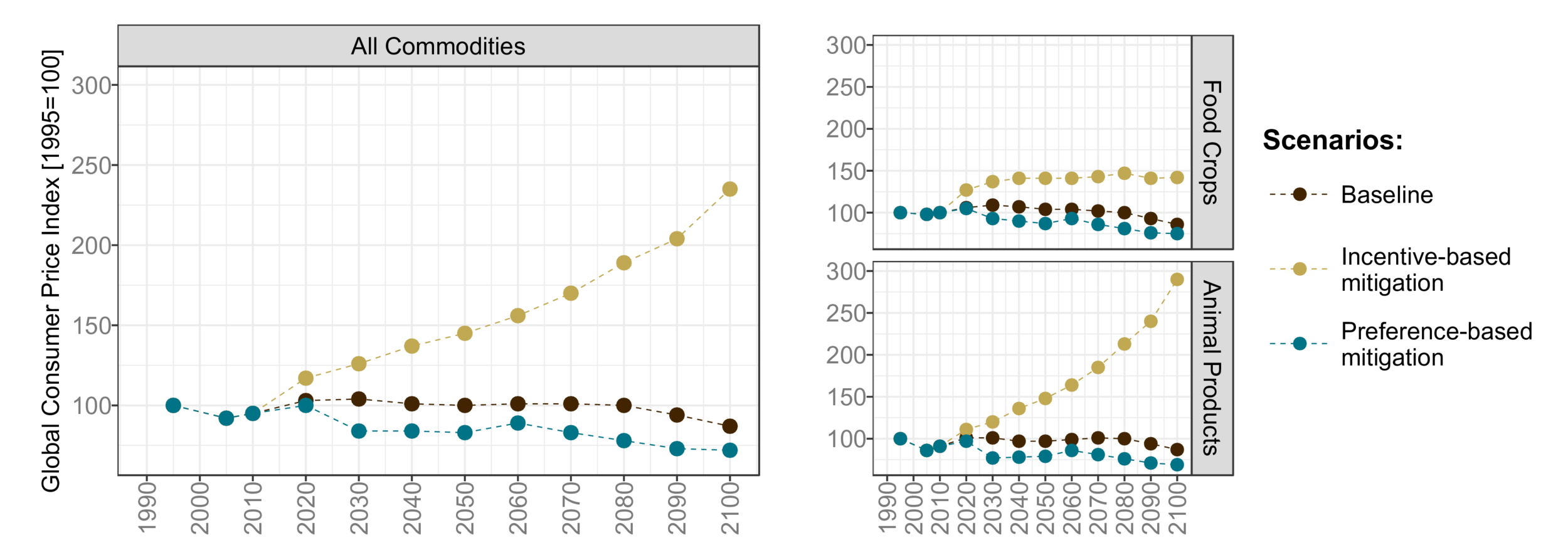
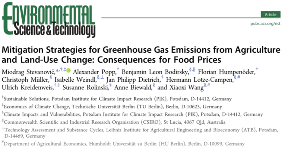
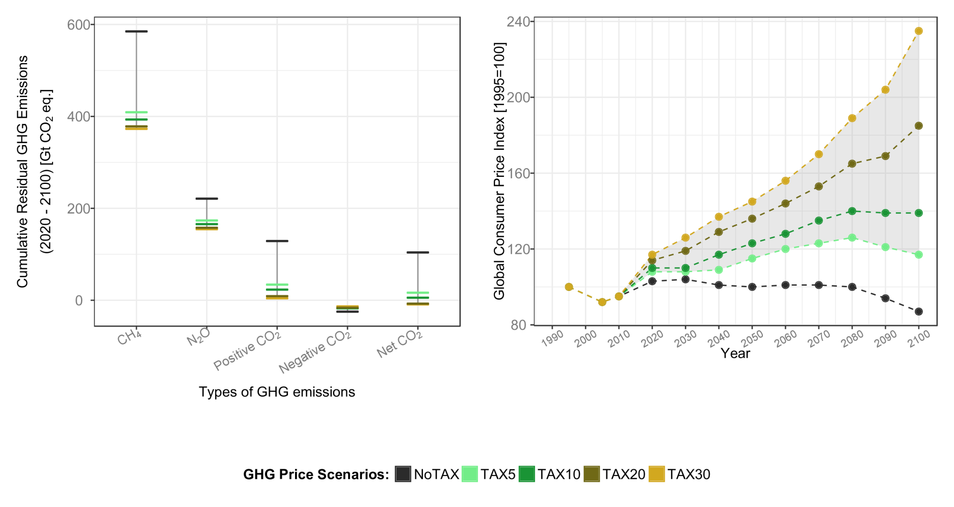
New features in 4

Flexible world regions


raw data
model input


ISO countries
MAgPIE v1-v3 world regions
Alternative aggregation
model input
powered by madrat » github.com/pik-piam/madrat
Standardized input processing


powered by madrat » github.com/pik-piam/madrat
retrieveData: bundle data as required by the model
readSource: read source data and (dis-)aggregate to ISO country level
calcOutput: calculate data sets as required by the model

Full modularization
MAgPIE 4
MAgPIE 3 beta
Extended model validation
powered by madrat » github.com/pik-piam/madrat
powered by mip » github.com/pik-piam/mip
Open Source


18 supporting R packages published under LGPL (copyleft) or BSD-2 (non-copyleft) Open Source license
github.com/pik-piam

In-code documentation
powered by goxygen » github.com/pik-piam/goxygen
[...]

*' @equations

*' ![Investment-yield ratio in relation to $\tau$-factor
*' [@dietrich_forecasting_2014]](tcc_regression.png){ width=60% }
*'
*' Relative technological change costs `v13_cost_tc` are calculated as a
*' heuristically derived power function of the land use intensity `vm_tau` for
*' the investment-yield-ratio (see figure above) multiplied by the current
*' regional crop areas `pc13_land` (taken from previous time step) and shifted
*' 15 years into the future using the region specific interest
*' rate `pm_interest`:

q13_cost_tc(i2) ..
  v13_cost_tc(i2) =e= sum(ct, pc13_land(i2) * i13_tc_factor(ct,i2)
                     * vm_tau(i2)**i13_tc_exponent(ct,i2)
                     * (1+pm_interest(i2))**15);

*' The shifting is performed because investments into technological change
*' require on average 15 years of research before a yield increase is achieved,
*' but the model has to see costs and benefits concurrently in order to take the
*' right investment decisions (see also @dietrich_forecasting_2014). Investment
*' costs are scaled in relation to crop area, since a wider areal coverage means
*' typically also higher variety in biophysical conditions, which would require
*' more research for the same overall intensity boost.
*'
*' In order to get the full investments required for the desired intensification
*' the relative technological change costs are multiplied with the given
*' intensification rate. These full costs are then distributed over an infinite
*' time horizon by multiplication with the interest rate `pm_interest(i)`
*' (annuity with infinite time horizon):

q13_tech_cost_annuity(i2) ..
 v13_tech_cost_annuity(i2) =e= (vm_tau(i2)/pc13_tau(i2)-1) * v13_cost_tc(i2)
                               * pm_interest(i2)/(1+pm_interest(i2));

*' Additionally, the technological change costs coming from past investment
*' decisions are added to the technological change costs of the current period:

q13_tech_cost(i2) ..
  vm_tech_cost(i2) =e= v13_tech_cost_annuity(i2) + pc13_tech_cost_past(i2);

[...]
Questions & Discussion
Further Reading
This presentation - slides.com/jandietrich/magpie-4-0
MAgPIE 4 framework paper - https://doi.org/10.5194/gmd-12-1299-2019
MAgPIE Repository | github.com/magpiemodel
R packages Repository | github.com/pik-piam
model requests | mxyzagpie@pik-poxyztsdam.de
contact me | dietrixyzch@pikxyz-potsdam.de


MAgPIE 4.0
By Jan Dietrich
MAgPIE 4.0
- 952
