Thermodynamics of structure-forming systems

Jan Korbel

CSH workshop

"Statistical Mechanical Approaches of Complex Systems"

17th-18th June 2024

slides available at: www.slides.com/jankorbel

other presentations: https://jankorbel.eu

Galore of entropies

Entropies

\(H = - \sum_i p_i \log p_i\)

\(R_q = \frac{1}{1-q} \ln \sum_i p_i^q \)

\(S_q = \frac{\sum_i p_i^q-1}{1-q}\)

\( S_{\alpha,\beta} = \sum_i \frac{p_i^\alpha-p_i^\beta}{\alpha-\beta}\)

\(S_{c,d} = \frac{\sum_i \Gamma(1+d,1-c \log p_i) -c}{1-c+cd} \) 

\(S_\phi = - \sum_i \int_{0}^{p_i} \log_\phi(x) \mathrm{d} x \) 

\(S_f = f^{-1} \left(\sum_i f(\ln p_i) \right)\)

\(S = k_B \log W\)

Boltzmann's entropy

\(S = k_B \log W\)

How to get there: https://stakata.wordpress.com/ludwig-boltzmann-and-myself/

Boltzmann's entropy for non-multinomial multiplicity

1. Maxwell-Boltzmann statistics with degeneracy

\(W(N_1,\dots,N_k) = N! \prod_{i=1}^k \frac{g_i^{N_i}}{N_i!}\)      \(S_{MB} = -  \sum_{i=1}^k p_i \log \frac{p_i}{g_i}\)

2. Bose-Einstein statistics

\(W(N_1,\dots,N_k) = \prod_{i=1}^k \binom{N_i + g_i-1}{N_i}\)

\(S_{BE} =  \sum_{i=1}^k  \left[(\alpha_i + p_i) \log (\alpha_i +p_i) - \alpha_i \log \alpha_i - p_i \log p_i\right]\)

3. Fermi-Dirac statistics

\(W(N_1,\dots,N_k) = \prod_{i=1}^k \binom{g_i}{N_i}\)

\(S_{FD} =  \sum_{i=1}^k  \left[-(\alpha_i - p_i) \log (\alpha_i -p_i) + \alpha_i \log \alpha_i - p_i \log p_i\right]\)

Entropy of structure-forming systems

• Many real-world systems form structures:
  • molecules of atoms
  • clusters of colloidal particles
  • (bio)polymers or micelles
  • social groups

• These systems are often described by grand-canonical ensemble

• The main feature is that the number of molecules is not conserved (it is the number of particles)

Is it appropriate?

Are we able to describe all phenomena?

Can we derive the canonical-ensemble entropy?

Structure-forming systems

Toy model - magnetic coin model

We consider a coin with two states: head             and tail

The coins are magnetic and can stick together 

How many states we get for N coins?

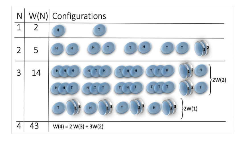
\(W(N) \sim N^N\)

(non-magnetic coins \(W(N) = 2^N\))

H. J. Jensen et al 2018 J. Phys. A: Math. Theor. 51 375002

Multiplicity of structure-forming  systems

Boltzmann entropy formula: \(S(n_i) = k_B \log W(n_i)\) 

where \(W\) is multiplicity

(number of microstates corresponding to a mesostate \(n_i\))

Microstate: state of each particle

       if more particles are bound to a molecule, then state of each molecule

Mesostate: how many particles and/or molecules are in given state

Example: magnetic coin model: 3 coins, magnetic

          microstates                        mesostate                 multiplicity

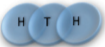
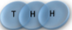
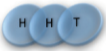
2 x           1x

1 x          1x

3

3

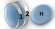
How to calculate a multiplicity?

1. Consider a mesostate
2. Make all permutations of particles
3. Some microstates are overrepresented - calculate how many permutations belong to the same microstate

Examples

2 x           1x

1 x          1x

1    1   2   2    3   3

2   3   1   3    1    2

3   2   3   1    2    1

1    1   2   2    3   3

2   3   1   3    1    2

3   2   3   1    2    1

= (1,2,3) , (2,1,3)

= (1,3,2) , (3,1,2)

= (2,3,1) , (3,2,1)

= (1,2,3) , (1,3,2)

= (2,1,3) , (2,3,1)

= (3,1,2) , (3,2,1)

General formula for multiplicity

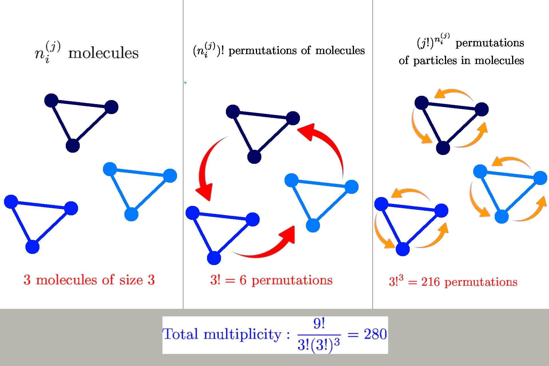
General formula: \(W(n_i^{(j)}) = \frac{n!}{\prod_{ij} n_i^{(j)}!  {\color{aqua} (j!)^{n_i^{(j)}}}}\)  

we have \(n_i^{(j)}\) molecules of size \(j\) in a state \(s_i^{(j)}\)

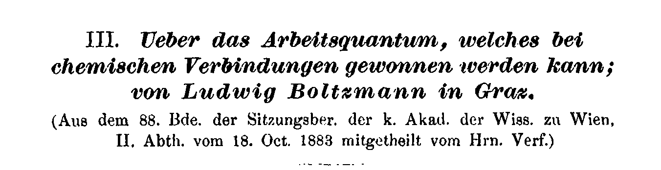
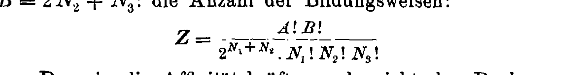
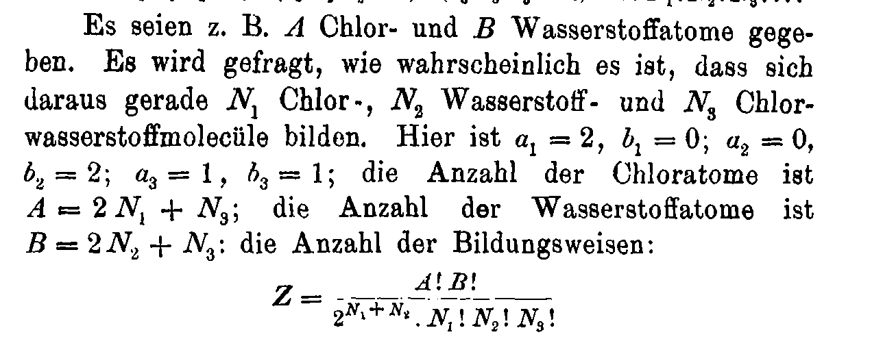
Boltzmann's 1884 paper

Entropy of structure-forming systems

We calculate the entropy from Boltzmann's formula using Stirling's approximation

$$ S =  \log W \approx n \log n - \sum_{ij} \left(n_i^{(j)} \log n_i^{(j)} - n_i^{(j)} + {\color{aqua} n_i^{(j)} \log j!}\right)$$

Introduce "probabilities" \(\wp_i^{(j)} = n_i^{(j)}/n\)

$$\mathcal{S} = S/n = - \sum_{ij} \wp_i^{(j)} (\log \wp_i^{(j)} {\color{aqua}- 1}) {\color{aqua}- \sum_{ij} \wp_i^{(j)}\log  \frac{j!}{n^{j-1}}}$$

Normalization: \( \sum_{ij} j \wp_i^{(j)} = 1\)

Finite interaction range: concentration \(c = n/b\) 

$$\mathcal{S} = S/n = - \sum_{ij} \wp_i^{(j)} (\log \wp_i^{(j)} {\color{aqua}- 1}) {\color{aqua}- \sum_{ij} \wp_i^{(j)}\log  \frac{j!}{{\color{orange}c^{j-1}}}}$$

Entropy of structure-forming systems

Main properties:

• The entropy fulfills Shannon Khinchin axioms 1,3,4 but does not fulfill axiom SK 2 (it is not maximized by uniform distribution)
• The entropy fulfills Lieb-Yngvason axioms (it is additive, and it is extensive for \(c=const\) )
• The entropy fulfills Shore-Johnson axioms 1,3,4 but does not fulfill axioms SJ 2 (permutation/coordinate invariance)
• The entropy fulfills Tempesta group-composability axiom but is not symmetric in its arguments
• The scaling exponents according to Hanel-Thurner axioms are                           \(c=0,d=1\), the same as for Shannon entropy

\( \Rightarrow\) The entropy satisfies all common axiomatic schemes but it is not symmetric in probabilities

$$\hat{\wp}_i^{(j)} = \frac{c^{j-1}}{j!} \exp(-\alpha j - \beta \epsilon_i^{(j)})$$

MaxEnt distribution

To find the MaxEnt distribution we define Lagrange functional

\(\mathcal{L}(\wp) = S(\wp) - \sum_{ij} j \wp_{i}^{(j)} - \beta \sum_{ij} \epsilon_i^{(j)} \wp_{i}^{(j)} \) 

By maximizing \(\mathcal{L}\) we obtain the MaxEnt distribution

This looks almost like the Boltzmann distribution, but there are a few differences

\(\sum_{ij} j \wp_i^{(j)} = \sum_{ij} \frac{c^{j-1}}{(j-1)!} e^{-{\color{aqua} \alpha} j - \beta \epsilon_i^{(j)}} = 1\) for \({\color{aqua} \alpha}\)

Normalization is not obtained by calculating the partition function but by solving

which is a polynomial equation in \(e^{-\alpha}\) of order equal to the maximum size of the molecule

Free energy and cluster-size distribution

Consequently, the free energy can be calculated as

\( F = U - \beta^{-1} S = - \frac{\alpha}{\beta} {\color{aqua}- \frac{\mathcal{M}}{\beta}}\)

where \(\mathcal{M} = \sum_{ij} \wp_{i}^{(j)}\) is the number of molecules (per particle)

If we focus only on the group-size distribution, we define

\( \wp^{(j)} = \sum_i \wp_i^{(j)}=e^{-j\alpha}  \mathcal{Z}_j\)

where \(\mathcal{Z}_j = \frac{c^{j-1}}{j!}\sum_i e^{-\beta \epsilon_i^{(j)}}\) is the partial partition function

We define the coarse-grained entropy 

\(S_c(\wp) = - \sum_j \wp^{(j)} (\log \wp^{(j)}-1)\)

and partial free energy \(F_j = -\beta^{-1} \ln \mathcal{Z}_j\)

The coarse-grained distribution can be obtained by maximizing  \(L_c(\wp) = S_c(\wp) - \beta \sum_j \wp_j F_j\) 

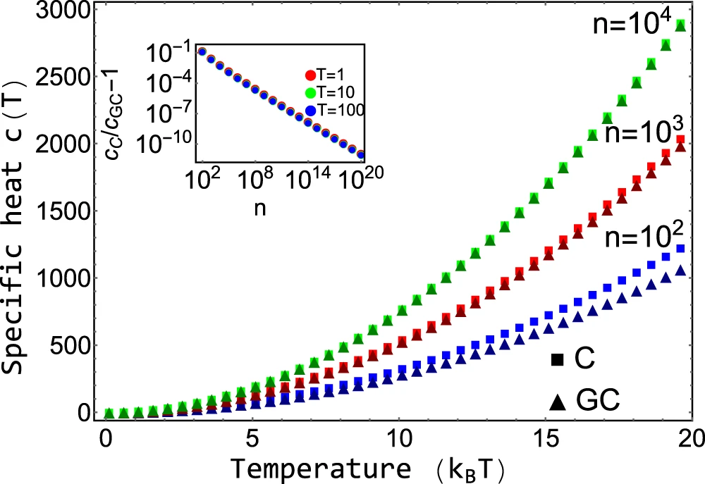
Comparison with grand-canonical ensemble

Stochastic thermodynamics of structure-forming systems

1. Linear Markov (= memoryless) with distribution \(\wp_i(t)\).

Its evolution is described by master equation

$$ \dot{\wp}_i(t) = \sum_{j} [w_{ij} \wp_{j}(t) - w_{ji} \wp_i(t) ]$$

\(w_{ij}\) is transition rate. 

2. Detailed balance

Assumptions

Stochastic thermodynamics of structure-forming systems

Results

1. Second law of thermodynamics for non-equilibrium systems

2. Detailed fluctuation theorem for structure forming systems

$$\frac{P(\Delta \sigma)}{\tilde{P}(-\Delta \sigma)} = e^{\Delta \sigma}$$

where  \(\Delta \sigma = \Delta s_i +  {\color{aqua} \log j_0 - \log j_f}\)

\(\Delta s_i\) is the trajectory entropy production

Applications

1. Self-assembly

 Self-assembly of Janus particles

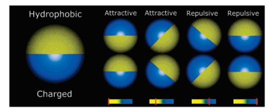
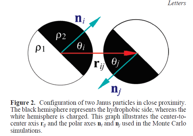
Kern-Frenkel model

Pair-wise potential: \(U^{KF}(r_{ij},n_i,n_j) = u(r_{ij}) \Omega(r_{ij},n_i,n_j) \)

Square-well interaction with hard sphere: 

$$ u(r_{ij}) = \left\{ \begin{array}{rl} \infty, & r_{ij} \leq \sigma \\  - \epsilon, & \sigma < r_{ij} < \sigma + \Delta \\ 0, & r_{ij} > \sigma + \Delta. \end{array} \right.$$

\(\Omega\) decribes orientation of particles:

Particle coverage \(\chi = \sin^2(\theta/2) = \frac{1-\cos{\theta}}{2}\)

Polymers: \(\chi = 0.3\)

Janus particles: \(\chi = 0.5\)

Crystalic structures: \(\chi = 0.6\) (stable lamellar crystals)

$$\Omega(r_{ij},n_i,n_j) = \left\{\begin{array}{rl} -1 & \mathrm{if} \  r_{ij} \cdot n_i > \cos(\theta) \ \mathrm{and} \ r_{ij} \cdot n_j > \cos(\theta)\\ 0 & \mathrm{otherwise} \end{array}  \right.$$

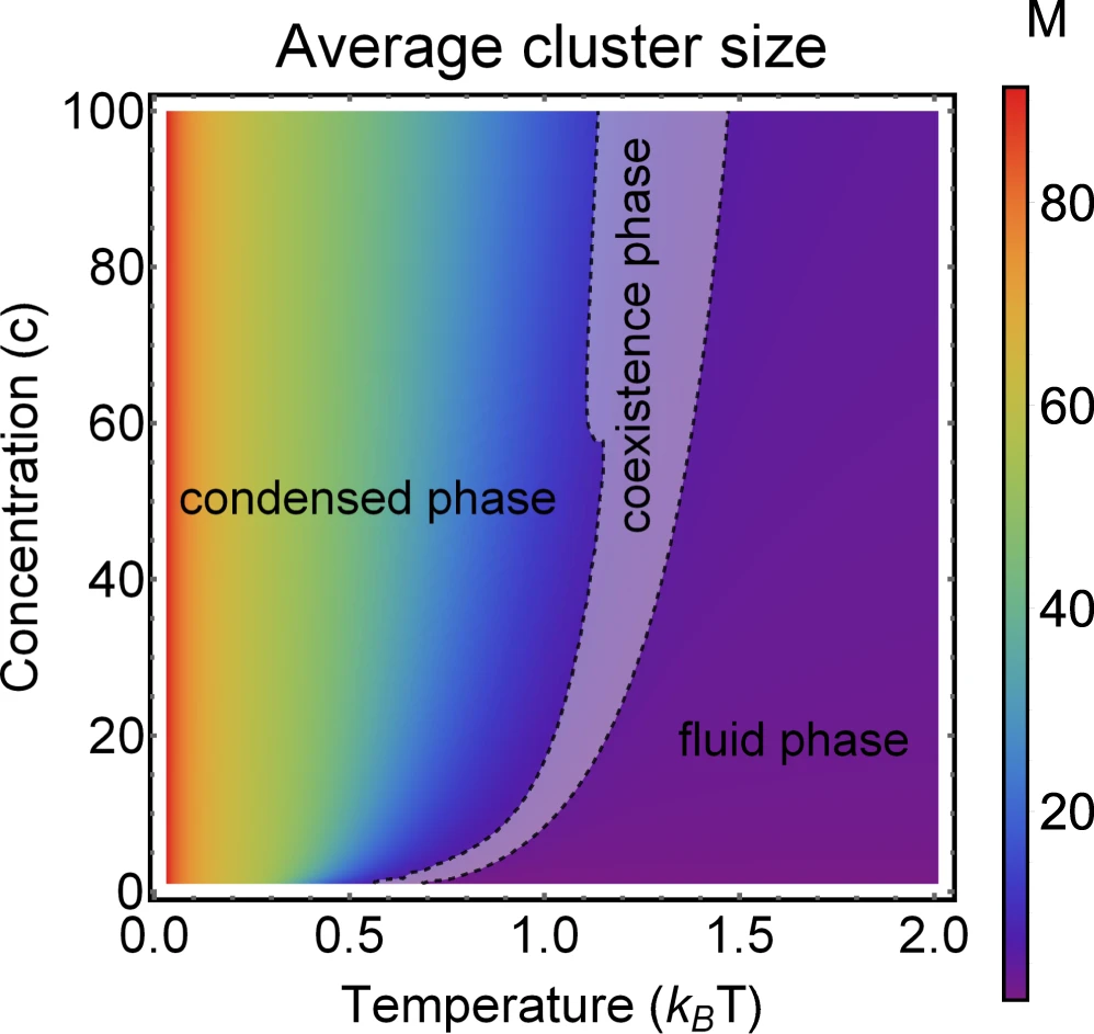
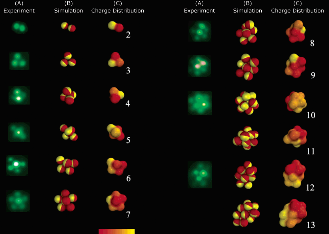
Phase diagram of Janus particles for average cluster size \(M\)

The phase diagram is in agreement with the known theory of self-assembly

2. Opinion dynamics

Driving forces in opinion dynamics

• Many opinion dynamics systems follow two basic concepts:

1. Homophily - people tend to be friends with peers with similar opinions
2.  Social balance - a friend of my friend is my friend, enemy of my friend is my enemy

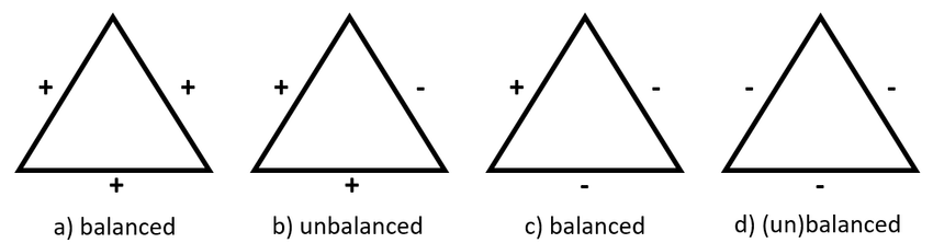
These two concepts can be related through the local Hamiltonian approach

Local Hamiltonian approach

• We introduce a local Hamiltonian (=local stress) based on homophily and show how it is related to social balance
• Each individual has \(G\) binary opinions, \(s_i \in \{-1,1\}^G\)
• If two connected individuals have more common opinions than different opinions, they become friends and vice versa \(J_{ij} = sign(s_i \cdot s_j)\)

Group formation based on homophily

Hamiltonian of a group \(\mathcal{G}\)

\(H(\mathbf{s}_{i_1},\dots,\mathbf{s}_{i_k}) =  \underbrace{- \phi \, \frac{J}{2} \sum_{ij \in \mathcal{G}} A_{ij} \mathbf{s}_i \cdot \mathbf{s}_j}_{\textcolor{red}{intra-group \ social \ stress}}+ \underbrace{(1-\phi) \frac{J}{2} \sum_{i \in \mathcal{G}, j \notin \mathcal{G}} A_{ij} \mathbf{s}_{i} \cdot \mathbf{s}_j}_{\textcolor{aqua}{inter-group \ social \ stress}} \\ \qquad \qquad \qquad \qquad - \underbrace{h \sum_{i \in \mathcal{G}} \mathbf{s}_i \cdot \mathbf{w}}_{external \ field}\)

Group formation based on opinion= self-assembly of spin glass

Group 1

Group 2

Approximations used in analytical calcualtions

1. Simulated annealing 

- We do not know the full network but just a degree distribution.  \(\Rightarrow\) The probability of observing a link between \(i\) and \(j\) is proportional to \(k_i k_j\)

2. Mean-field approximation

- We use the mean-field approximation of the Hamiltonian

\(\Rightarrow\)  \(m^{(k)} = \sum_{i \in group \ of \ size \ k} s_i\) -  average opinion vector of a group of size \(k\)

These two approximations lead to the set of self-consistency equations:

$$m^{(k)} = k \sum_{q^{(k)} q^{(k,l)}} P(q^{(k)}) P(q^{(k,l)}) \tanh(\beta H^{(k)}(m^{(l)},q^{(k)},q^{(k,l)})) $$

where \(q^{(k)}\) is the intra-group degree, \(q^{(k,l)}\) is the inter-group degree and \(P\) is the degree distribution

Results for zero inter-group degree

Theory

MC simulation

Dependence on external field

Application online multiplayer game PARDUS

3. Phase transitions in systems with several interactions

Phase transitions of systems

with multiple interactions

• Many real-world systems (both natural and socio-economic) exhibit phase transitions
• The order of the phase transition depends on the type of interaction
• As shown in several recent studies, the transition between first-order and second-order transition is typically happening in systems with more than one type of interaction
• We will focus on the systems, where one type of the interaction is not energetic, but rather "entropic" (i.e., arises from non-multinomial multiplicity)

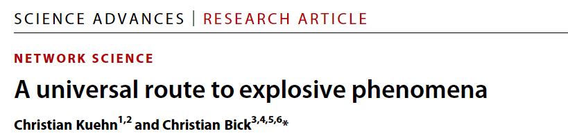
Toy model - Ising model with molecule formation

Multiplicity of structure-forming systems

• For the model, we derive the multiplicity of a state \(\{n_\uparrow,n_\downarrow,n_\|\}\) 
• The normalization is \(n_\uparrow+n_\downarrow+ 2 n_\| = n\)
• It can be derived as \(W(n_\uparrow,n_\downarrow,n_\|) = \Omega(n_\uparrow,n_\downarrow,n_\|) M(n_\|) \)
• Here, \(\Omega(n_\uparrow,n_\downarrow,n_\|) = \binom{n}{n_\uparrow \ n_\downarrow \ 2 n_\|}\) is the multinomial factor representing the number of divisions of \(n\) particles into the states of the system
• \(M(n_\|)\) represents the number of ways that \(2 n_\|\) particles can form \(n_\|\) molecules
• In fully-connected network, we know it is equal to $$M(n_\|) =  \frac{(2 n_\|)!}{(n_\|)! 2^{n_\|}}$$

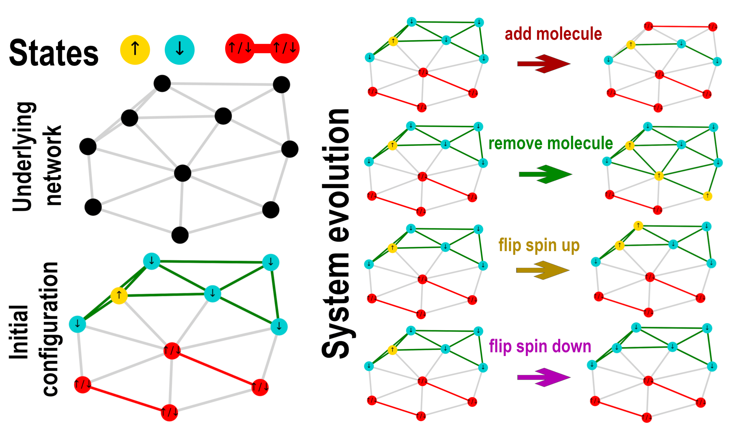
Multiplicity on random network

By using the procedure above, we can show that the multiplicity is $$M(n_\|) = \frac{1}{(n_\|)!} \prod_{i=0}^{n_\|-1} L(2n_\|-2i)$$

• For each step, we can approximate the number of links by             \(L =  k/(2n)\) where \(k\) is the average degree
• By using this approximation, we end with

$$M(n_\|) =  \frac{(2n_\|)!}{n_\|!} \left(\frac{k}{2(n-1)}\right)^{n_\|} $$

Entropy of Ising model with molecules

• Subsequently, the entropy can be expressed as $$S \equiv \log W = \log (\Omega M)$$ which leads to $$S(\wp_\uparrow,\wp_\downarrow,\wp_\|) = - \wp_\uparrow (\log \wp_\uparrow - 1) - \wp_\downarrow (\log \wp_\downarrow - 1)$$  $$- \wp_\| (\log \wp_\| - 1)- \wp_\| \log \left(\frac{2(n-1)}{k n}\right) $$ where \(\wp_i = n_i/n\)

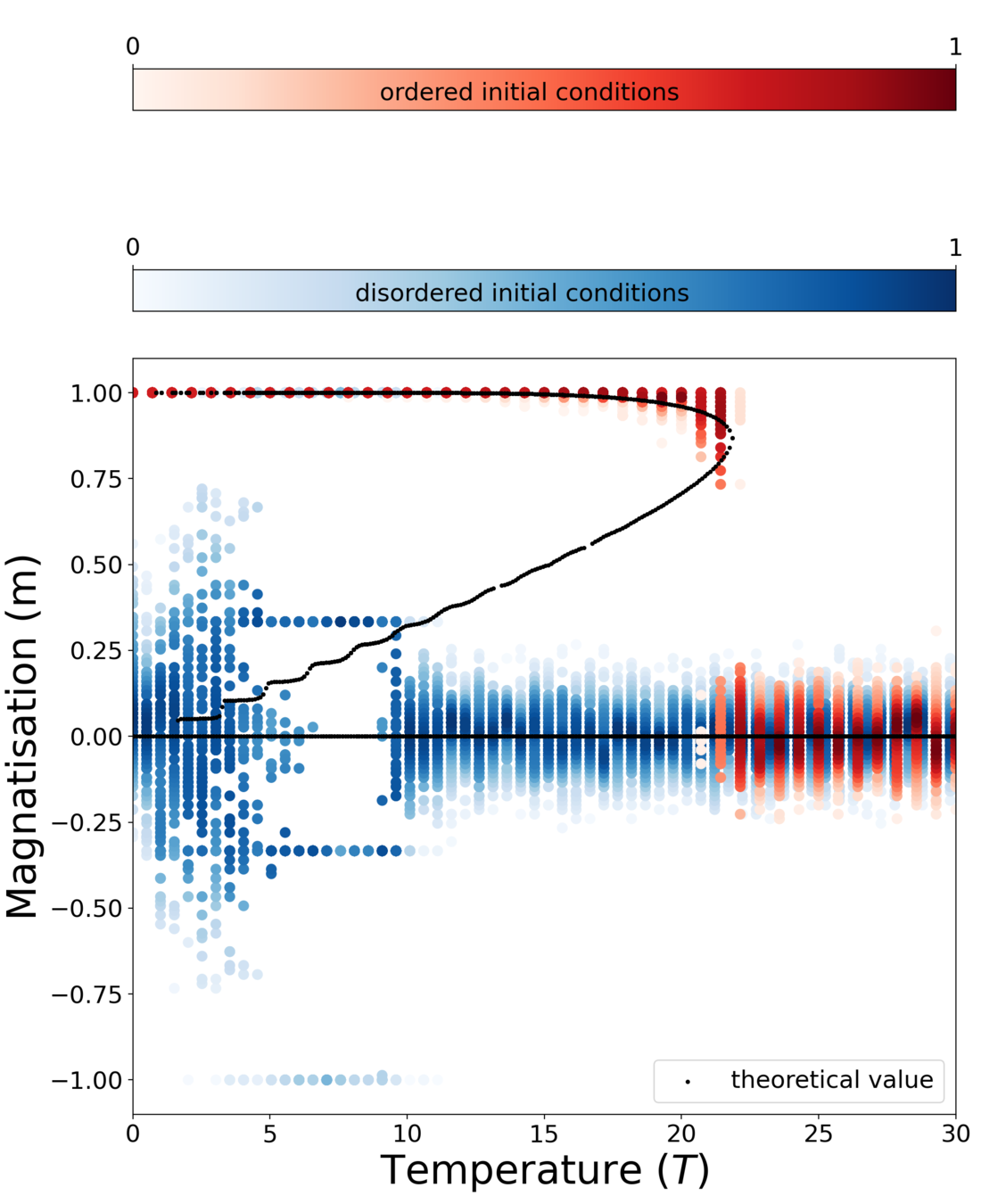
Self-consistency equation

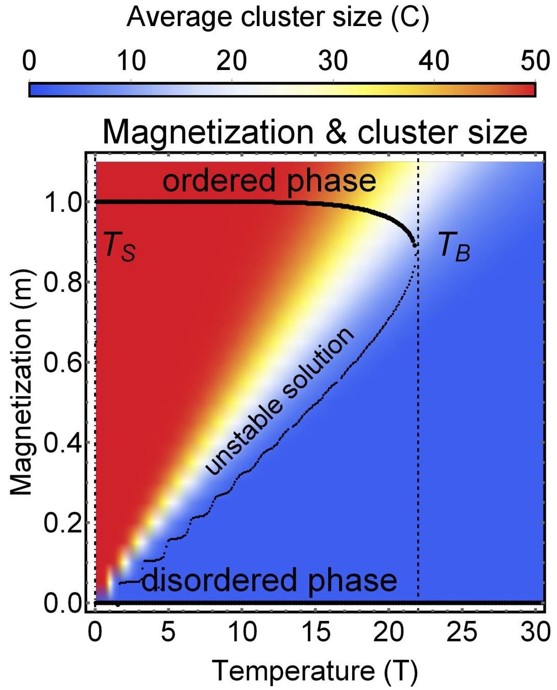
• Using the Ising-like Hamiltonian \(H(s) = - \frac{1}{k} \sum_{ij} A_{ij} s_i s_j\) where \(A_{ij}\) is the adjacency matrix, and with formally setting \(s_\|=0\) we can derive (in the mean-field approximation with configuration model) the following self-consistency equation $$m =   \frac{2 \left(- \cosh( \beta J m) + \sqrt{  \cosh^2(\beta J m) + k}\right)}{k} \sinh (\beta J m )$$
• By using the Taylor expansion, we can show that the for \(k\leq 8\) we observe the second-order transition, for \(k>8\) we can observe the first-order transition
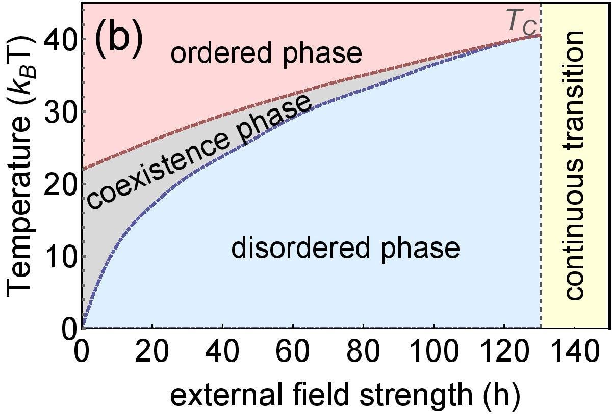
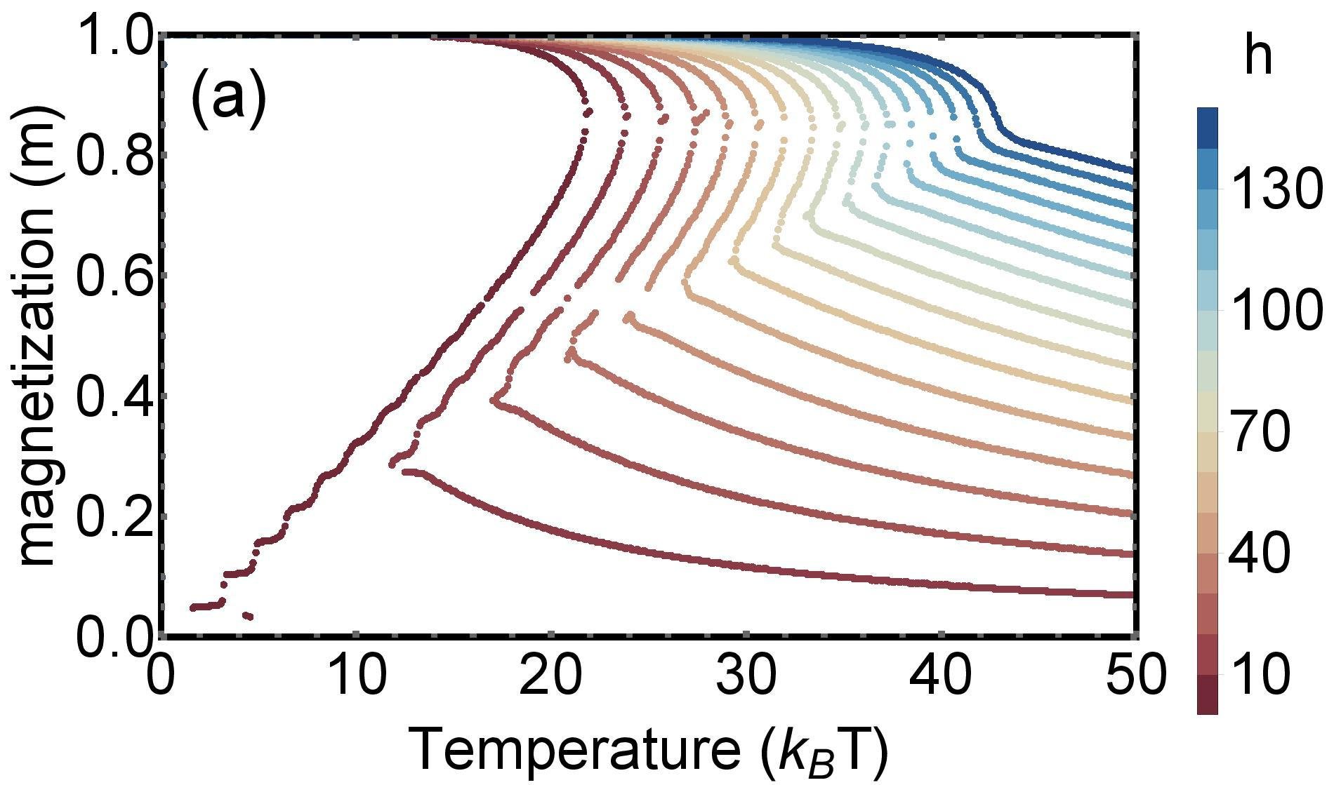
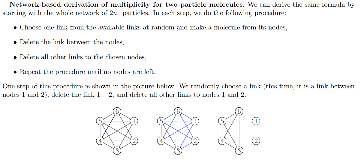
• We can also consider that only a fraction of \(q\) particles can form molecules - then we obtain a rich phase diagram

Phase diagram

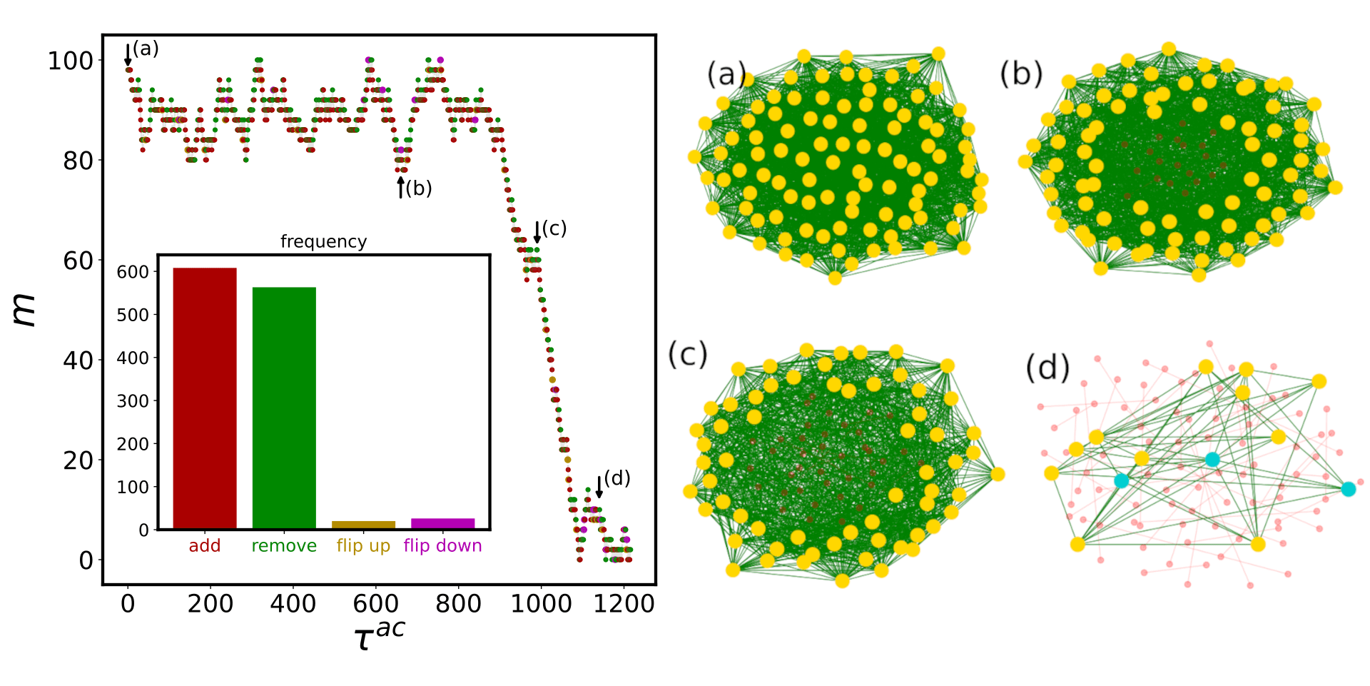
Mechanism - microscopic transtions

Thank you for your attention