USING STOCHASTIC THERMODYNAMICS TO ANALYZE NON-THERMODYNAMIC PROPERTIES OF DYNAMIC SYSTEMS

QLS meeting, 12th July 2022

in collaboration with

Tuan Pham

Farita Tasnim

David Wolpert

USING STOCHASTIC THERMODYNAMICS TO ANALYZE NON-THERMODYNAMIC PROPERTIES OF DYNAMIC SYSTEMS

OUTLINE

 

• Stochastic thermodynamics for non-physical systems          (motivation a.k.a. big picture)

• ​Stochastic thermodynamics of dynamic opinion networks and genetic regulatory networks                                                      (detailed example of ST for non-physical systems)

Why stochastic thermodynamics in non-physical systems? 

What do non-physical systems have in common with the typical setup of stochastic thermodnyamics?

Linear Markov evolution of probability distribution

\( \dot{p}_m(t) = \sum_n (w_{mn} p_n(t) - w_{nm} p_m(t)) \)

This has profound consequences. Regardless of any physical interpretation, the entropy production rate

\( \dot{\Sigma}_t = \sum_{mn} (w_{mn} p_n - w_{nm} p_m ) \log \frac{w_{mn} p_n}{w_{nm} p_m} \)

is a non-negative quantity. Many results of ST including

\( \frac{P(\bar{\Sigma}_t = A)}{\tilde{P}(\bar{\Sigma}_t= -A)} = e^{At} \)

FT's

\(\frac{Var(J_t)}{E(J_t)^2} \geq \frac{2}{\bar{\Sigma}_t}\)

TUR's

\(\frac{L(p(t),p(0))}{2 \Sigma_t \bar{A}_t} \leq t\)

SLT's

are still valid.

Similarities

DIFFERENCES

What ARE DIFFERENCES BETWEEN  NON-PHYSICAL SYSTEMS AN typical setup of stochastic thermodnyamics?

Broken local detailed balance

\(\log \frac{w_{mn}}{w_{nm}} \neq \beta (\epsilon_m - \epsilon_n)\)

That's OK. Many results of ST still remain valid.

 

No existence of a single potential (energy)

state \(m \nRightarrow\) energy \( \epsilon_m\)

No global first law of thermodynamics.

While the physical interpretation of the second law is not valid anymore, its applications to ST remain valid.

TYPICAL SETUP OF

NON-PHYSICAL SYSTEMS

subsystem 1

states \(s_i^1\)

potential \( H^1(s_i^1|\textcolor{green}{s_j^2})\)

subsystem LDB

\(\log \frac{w_{ii'}^1}{w_{i'i}^1} = \beta^1(H^1(s_i^1|\textcolor{green}{s_j^2}) - H^1(s^1_{i'}|\textcolor{green}{s_j^2}))\)

subsystem 2

states \(s_i^2\)

potential \( H^2(s_i^2|\textcolor{blue}{s_j^1})\)

subsystem LDB

\(\log \frac{w_{ii'}^2}{w_{i'i}^2} = \beta^2(H^2(s_i^2|\textcolor{blue}{s_j^1}) - H^2(s^2_{i'}|\textcolor{blue}{s_j^2}))\)

No global potential

No global LDB

TYPICAL SETUP OF

NON-PHYSICAL SYSTEMS

Does existence of subsystem potentials (Hamiltonians) lead to existence of global potential?

1

2

3

4

5

Generally not. Subsystem potentials must satisfy certain constraints.

 

EXamples OF

NON-PHYSICAL SYSTEMS

1) lIVING systems

The simplest model of a living system

metabolism

nutrients

energy

ATP

chemical reaction network

energy \(E_n\)

# molecules \(N_n\)

evolution

genotype

phenotype

fitness function \(\Psi_n\)

environment

ATP synthase

...

EXamples OF

NON-PHYSICAL SYSTEMS

2) Distributed computational systems

by Farita Tasnim

a) parallel bit erasure

b) modularity of computational systems

c) hierarchy of computational systems

d) as a result, computational systems have a similar structure

 

EXamples OF

NON-PHYSICAL SYSTEMS

3) OPINION DYNAMICS OF SOCIAL NETWORKS

influencer

followers

friends

influencer

followers

friends

friends

opinions \(s_i\), local stress function \(H^i(s_i|s_j)\)

SIMPLE EXAMPLE of A system with Local potentials driven by CTMC 

• Consider a system compound of N subsystems
• Each subsystem has a binary state \(s_i \in \{-1,1\}\)
• The coupling between subsystems is given by (possibly asymmetric) matrix \(J_{ij} \in \{0,1\}\)
• We define the in-neighborhood of a subsystem \(i\) as \(N_i = \{j|J_{ij} = 1\}\)
• Local Hamiltonian is defined as \(H^i(s_i|s_j) = - \sum_{j \in N_i} s_i s_j\)
• The systems evolves according to CTMC (master equation) $$ p(\vec{s}) = \sum_{\vec{s}'} w_{\vec{s}\vec{s}'} p(\vec{s}')$$
• The rate matrix can be decomposed as \( w_{\vec{s}\vec{s}'} = \sum_i w^i_{\vec{s}\vec{s}'}\) where \(w^i_{\vec{s}\vec{s}'}\) is non-zero only if \(s_j = s_j'\) for \(j \neq i\) (i.e., \(w^i\) is the rate matrix for i-th subsystem)
• We consider subsystem local detailed balance $$\log \frac{w^i_{\vec{s}\vec{s}'}}{w^i_{\vec{s}'\vec{s}}} = \beta (H^i(\vec{s}')-H^i(\vec{s}))$$
• The whole dynamics and thermodynamics is given by the network topology (and initial conditions)

local ising spin hamiltonian model

influencer

followers

friends

influencer

followers

friends

friends

opinions \(s_i\), local stress function \(H^i(s_i|s_j)\)

local ising spin hamiltonian model

=OPINION DYNAMICS OF A SOCIAL NETWORK

local ising spin hamiltonian model

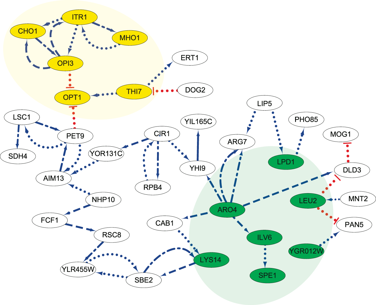
=SIMPLE MODEL OF A GENE REGULATORY NETWORK

What is the dependence of Entropy production on network topology?

In general: the dependence of EP on network topology is complicated. 

Experiment: start with a directed acyclic graph and try to

                         a) add more links

                         b) make some links reciprocal

Question: what is the impact on entropy production?

                     what is the impact on adiabatic and non-adiabatic EP?

 

$$ \dot{\Sigma}^{a}_t = \sum_{mn} (w_{mn}p_n - w_{nm} p_m) \log \frac{w_{mn}p^{st}_n}{w_{nm}p^{st}_m}$$

$$ \dot{\Sigma}^{na}_t = \sum_{mn} (w_{mn}p_n - w_{nm} p_m) \log \frac{p^{st}_n}{p^{st}_m}$$

 

What is the dependence of Entropy production on network topology?

MORE RESULTS

Speed limit theorems

MORE RESULTS

THERMODYNAMIC UNCERTAINTY RELATIONS

SUMMARY

• Many results of stochastic thermodynamics can be useful in non-physical systems
• These systems are typically composed of many subsystems
• While each subsystem is described by local potential (Hamiltonian) and satisfied subsystem local detailed balance, there is no global Hamiltonian (and no global LDB)
• Dependence of thermodynamic quantities on network topology is quite complicated, however, some preliminary results were obtained