Foundations of Entropy II

 

 Let's calculate 'em

 

 

Lecture series at the 

School on Information, Noise, and Physics of Life

Nis 19.-30. September 2022

 

by Jan Korbel

all slides can be found at: slides.com/jankorbel

Activity II

 

You have 3 minutes to write down on a piece of paper:

             

             What is the most unexpected/surprising application

of entropy

             you have seen? (unexpected field, unexpected result)

 

 

 

 

Using Boltzmann's formula for non-multinomial systems

As we saw in the previous lecture, the multinomial multiplicity

$$W(n_1,\dots,n_k) = \binom{n}{n_1,\dots,n_k}$$

leads to Boltzmann-Gibbs-Shannon entropy.

 

 

Are there systems with non-multinomial multiplicity?

What is their entropy?

Ex. I: MB, FD & BE statistics

1. Maxwell-Boltzmann statistics - \(N\) distinguishable particles, \(N_i\) particles in state \(\epsilon_i\)

Multiplicity can be calculated as

$$W(N_1,\dots,N_k) = \binom{N}{N_1} \binom{N-N_1}{N_2} \dots \binom{N-\sum_{i=1}^{k-1}N_1}{N_k} = N! \prod_{i=1}^k \frac{1}{N_i!}$$

If \(\epsilon_i\) has degeneracy \(g_i\), then

$$W(N_1,\dots,N_k) = N! \prod_{i=1}^k \frac{g_i^{N_i}}{N_i!}$$

Then, we get

$$S_{MB} = - N \sum_{i=1}^k p_i \log \frac{p_i}{g_i}$$

Ex. I: MB, FD & BE statistics

2. Bose-Einstein statistics - \(N\) indistinguishable particles, \(N_i\) particles in state \(\epsilon_i\) with  degeneracy \(g_i\),

 

Multiplicity can be calculated as

$$W(N_1,\dots,N_k) = \prod_{i=1}^k \binom{N_i + g_i-1}{N_i}$$

Let us introduce \(\alpha_i = g_i/N\). Then, we get

$$S_{BE} = N \sum_{i=1}^k  \left[(\alpha_i + p_i) \log (\alpha_i +p_i) - \alpha_i \log \alpha_i - p_i \log p_i\right]$$

(|*)

3. Fermi-Dirac statistics - \(N\) indistinguishable particles, \(N_i\) particles in state \(\epsilon_i\) with  degeneracy \(g_i\), maximally 1 particle per sub-level (thus \(N_i \leq g_i\))

 

Multiplicity can be calculated as

$$W(N_1,\dots,N_k) = \prod_{i=1}^k \binom{g_i}{N_i}$$

Let us introduce \(\alpha_i = g_i/N\). Then, we get

$$S_{FD} = N \sum_{i=1}^k  \left[-(\alpha_i - p_i) \log (\alpha_i -p_i) + \alpha_i \log \alpha_i - p_i \log p_i\right]$$

Ex. I: MB, FD & BE statistics

Ex. II: structure-forming systems

Let us start with a simple example of a coin tossing.

States are:  

But! let's make a small change, we consider magnetic coins

The bound (or sticky) state is simply  

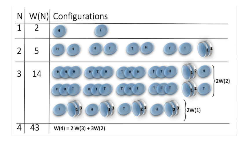
State space grows super-exponentially  (\(W(n) \sim n^n \sim e^{n \log n}\) )

picture taken from: Jensen et al 2018 J. Phys. A: Math. Theor. 51 375002

Multiplicity

2 x           1x

1 x          1x

3

3

Microstate

Mesostate

Mesostate

2 x           1x

1 x          1x

1    1   2   2    3   3

2   3   1   3    1    2

3   2   3   1    2    1

 

1    1   2   2    3   3

2   3   1   3    1    2

3   2   3   1    2    1

 

= (1,2,3) , (2,1,3)

= (1,3,2) , (3,1,2)

= (2,3,1) , (3,2,1)

= (1,2,3) , (1,3,2)

= (2,1,3) , (2,3,1)

= (3,1,2) , (3,2,1)

How to calculate multiplicity

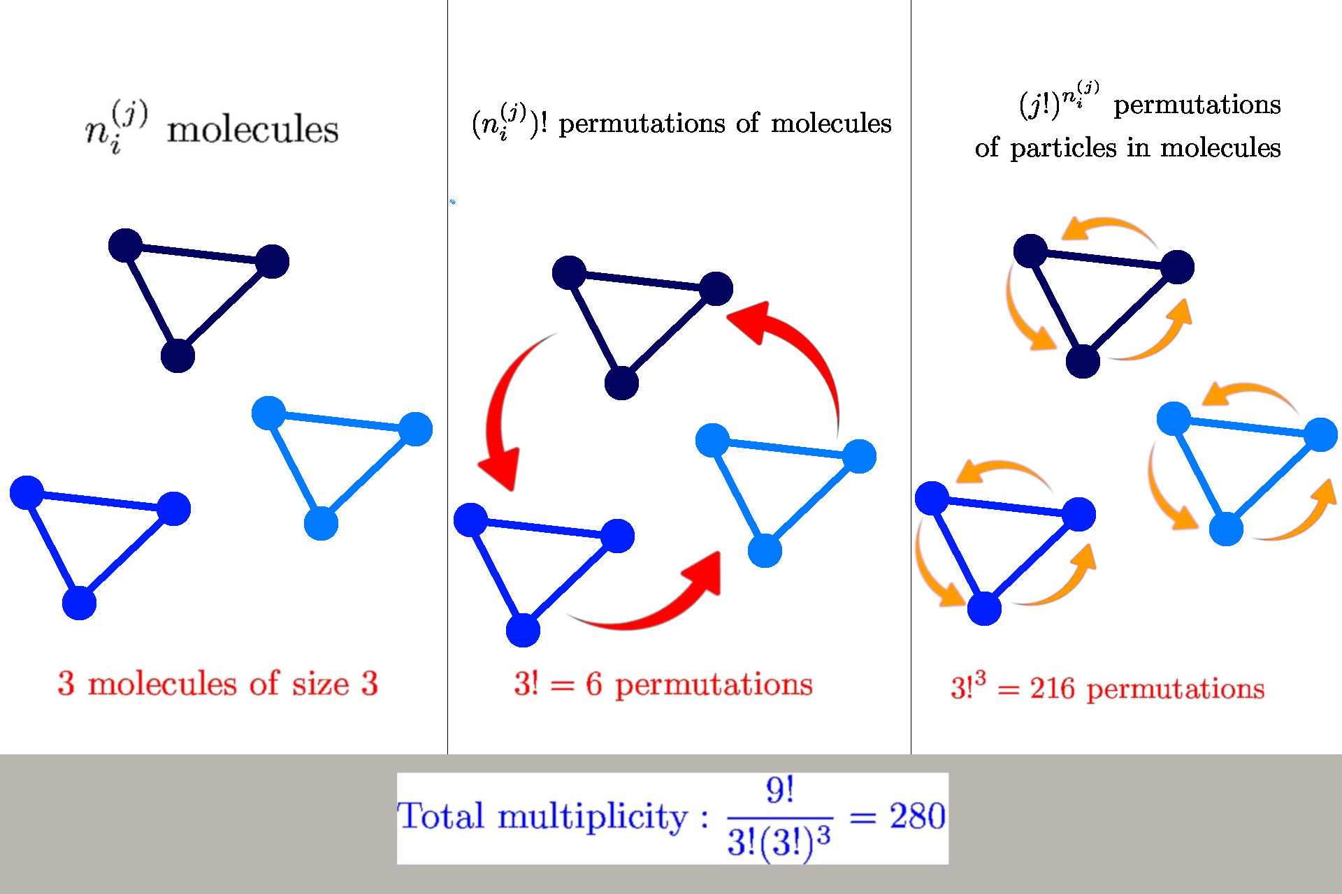
General formula: \(W(n_i^{(j)}) = \frac{n!}{\prod_{ij} n_i^{(j)}!  {\color{red} (j!)^{n_i^{(j)}}}}\)  

we have \(n_i^{(j)}\) molecules of size \(j\) in a state \(s_i^{(j)}\)

Multiplicity

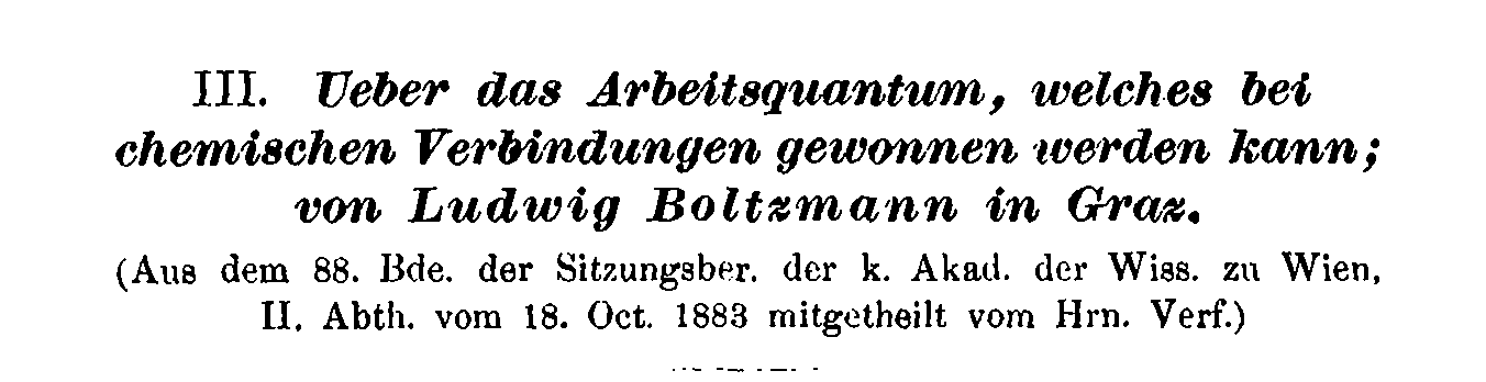
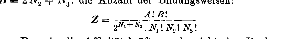
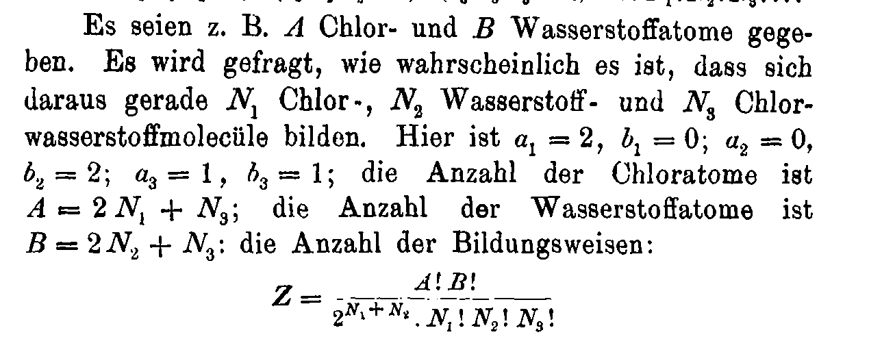
Boltzmann's 1884 paper

Entropy of structure-forming systems

$$ S =  \log W \approx n \log n - \sum_{ij} \left(n_i^{(j)} \log n_i^{(j)} - n_i^{(j)} + {\color{red} n_i^{(j)} \log j!}\right)$$

Introduce "probabilities" \(\wp_i^{(j)} = n_i^{(j)}/n\)

$$\mathcal{S} = S/n = - \sum_{ij} \wp_i^{(j)} (\log \wp_i^{(j)} {\color{red}- 1}) {\color{red}- \sum_{ij} \wp_i^{(j)}\log  \frac{j!}{n^{j-1}}}$$

Finite interaction range: concentration \(c = n/b\) 

$$\mathcal{S} = S/n = - \sum_{ij} \wp_i^{(j)} (\log \wp_i^{(j)} {\color{red}- 1}) {\color{red}- \sum_{ij} \wp_i^{(j)}\log  \frac{j!}{{\color{purple}c^{j-1}}}}$$

 

 Nat. Comm. 12 (2021) 1127

Ex. III: sample-space reducing processes (SSR)

 Corominas Murtra, Hanel, Thurner PNAS 112(17) (2015) 5348

Multiplicity

The number of states is \(n\). Let us denote the states as \(x_n \rightarrow \dots \rightarrow x_1\), where \(x_1\) is the ground state, where the process restarts. Let us sample \(R\) relaxation sequences \(x = (x_{k_1},\dots,x_1)\). 

The sequences can be visualised as

 

 

 

 

 

 

 

How many of these sequences contain  a state \(x_{j}\) exactly \(k_j\) times?  

Each run must contain \(x_1\)

Multiplicity

Number or runs \(R \equiv k_1\), number of them containing \(x_j\) is \(k_j\)

Multiplicity of these sequences: \(\binom{k_1}{k_j}\)

By multiplying the multiplicity for each state we get

$$W(k_1,\dots,k_n) = \prod_{j=2}^n \binom{k_1}{k_j}$$

$$ \log W \approx \sum_{j=2}^n \left[k_1 \log k_1 - \cancel{k_1} - k_j \log k_j + \cancel{k_j} - (k_1-k_j) \log (k_1 - k_j) + \cancel{(k_1-k_j)}\right]$$

$$\approx \sum_{j=2}^n \left[ k_1 \log k_1 \textcolor{red}{-k_j \log k_1} - k_j log \frac{k_j}{\textcolor{red}{k_1}} - (k_1-k_j) \log(k_1-k_j) \right]$$

By introducing \(p_i = k_i/N\) where \(N\) is the total number of steps, we get

$$S_{SSR}(p) = - N \sum_{j=2}^n \left[p_i \log \left(\frac{p_i}{p_1}\right) + (p_1-p_i) \log \left(1-\frac{p_i}{p_1}\right)\right]$$

Ex. IV: Pólya urns

Hanel, Corominas Murtra, Thurner New J. Phys. (2017) 19 033008

Probability of a sequence 

We have  \(c\) colors, initially \(n_i(0) \equiv n_i\) balls of color \(c_i\). After a ball is drawn, we return \(\delta\) balls of the same color to the urn.

After \(N\) draws, the number of balls in the urn is

$$n_i(N) = n_i + \delta k_i$$

where \(k_i\) is the number of draws of color \(c_i\). The total number of balls is \(n(R) = \sum_{c} n_c(N) = N + \delta N\) 

The probability of drawing a ball of color \(c_i\) in \(N\)-th run, is \(p_i(N) = n_i(N)/n(N)\). The probability of sequence

\(\ \mathcal{I} =\{i_1,\dots,i_N\} \) is 

$$p(\mathcal{I}) = \prod_{j=1}^c \frac{n_{j}^{(\delta,k_j)}}{n^{(\delta,N)}}$$

where \(m^{(\delta,r)} = m(m+\delta)\dots(m+r\delta)\) 

Probability of a histogram

A histogram \(\mathcal{K} = \{k_1,\dots,k_c\}\) is defined as \(k_c = \sum_{j = 1}^N \delta(i_j,c) \)

Thus the probability of observing a histogram is

$$ p(\mathcal{K}) =  \binom{N}{k_1,\dots,k_c} p(\mathcal{I}) $$ 

\(n_{j}^{(\delta,k_{j})} \approx k_{j}! \delta^{k_{j}}  (k_i+1)^{n_i/\delta} \) 

\( p(\mathcal{K}) = \frac{N!}{\prod_{j=1}^c \cancel{k_j!}} \frac{\prod_{j=1}^c \cancel{k_j!} \delta^{k_j} (k_j+1)^{n_j/\delta}}{n^{(\delta,N)}} \)

... technical calculation ...

 

$$S_{Pólya}(p) = \log p(\mathcal{K}) \approx - \sum_{i=1}^c \log(p_i + 1/N)$$

Ex. IV: q-deformations

This example is rather theoretical, but provides us a useful hint of what happens if there are correlations in the sample space

Motivation: finite versions of \(\exp\) and \(\log\)

\(\exp(x) = \lim_{n \rightarrow \infty} \left(1+\frac{x}{n}\right)^n\)

So define

\(\exp_q(x) := \left(1 + (1-q) x\right)^{1/(1-q)}\)

\(\log_q(x) := \frac{x^{1-q}-1}{1-q}\)

Let us find an operation s.t.

\(\exp_q(x) \otimes_q \exp_q(y) \equiv \exp_q(x+y)\)

\(\Rightarrow a \otimes_q b = \left[a^{1-q} + b^{1-q}-1\right]^{1/(1-q)}\)

Suyari, Physica A 368 (2006) 63-82

Calculus of q-deformations

In analogy to \(n! = 1 \cdot 2 \cdot \dots \cdot n\) introduce \(n!_q := 1 \otimes_q 2 \otimes_q  \dots \otimes_q n\)

It is than easy to show that \(\log_q n!_q = \frac{\sum_{k=1}^n k^{1-q} - n}{1-q}\) which can be used for generalized Stirling's approximation \(\log_q n!_q \approx \frac{n}{2-q} \log_q n\)

Let us now consider a q-deformed multinomial factor

$$\binom{n}{n_1,\dots,n_k}_q := n!_q \oslash_q (n_1!_q \otimes_q \dots \otimes_q n_k!_q) $$

$$ =  \left[\sum_{l=1}^n l^{1-q} - \sum_{i_1}^{n_1} i_i^{1-q} - \dots - \sum_{i_k}^{n_k} i_k^{1-q}\right]^{1/(1-q)}$$

 

Tsallis entropy

Let us consider that the multiplicity is given by a q-multinomial factor \( W(n_1,\dots,n_k) = \binom{n}{n_1,\dots,n_k}_q\)

 

In this case, it is more convenient to define entropy as \(S = \log_q W\), which gives us:

 

$$\log_q W = \frac{n^{2-q}}{2-q} \frac{\sum_{i=1}^k p_i^{2-q}-1}{q-1} = \frac{n^{2-q}}{2-q} S_{2-q}(p)$$

This entropy is known as Tsallis entropy

Note that the prefactor is not \(n\) but \(n^{2-q}\)

(non-extensivity) - we will discuss this later

Entropy and energy

 

Until now, we have been just counting states; let us now discuss the relation with energy. 

 

We consider that the states describe the energy of the system (either Hamiltonian or more generalized energy functional)

 

Therefore, entropy is defined as

$$ S(E) := \log W(E)$$

Ensembles

There are a few typical situations:

1. Isolated system = microcanonical ensemble

Let \(H(s)\) be the energy of a state \(s\). Multiplicity is then \(W(E) = \sum_{s} \delta(H(s) - E)\)

Phenomena like negative "temperature" \(T = \frac{\mathrm{d} S(E)}{\mathrm{d} E} < 0\)

2. closed system = canonical ensemble

Total system is composed of the system of interest (S) and the heat reservoir/bath (B). They are weakly coupled i.e., \(H_{tot}(s,b) = H_S(s) + H_B(b)\) (no interaction energy)

$$W(E_{tot}) = \sum_{s,b} \delta(H_{tot}(s,b) -E_{tot})$$

3. open system = grandcanonical ensemble

This can be further rewritten as 

$$= \int \mathrm{d} E_S\,  \sum_s \delta (H_{S}(s)-E_S) \sum_b(H_B(b)-(E_{tot}-E_S)) $$

$$= \int \mathrm{d} E_S \, W_S(E_S) W_B(E_{tot}-E_S) $$

Entropy in canonical ensemble

This is hard to calculate. Typically, the dominant contribution is from the maximal configuration of the integrand, which we obtain from 

$$\frac{\partial W_S(E_S) W_B(E_{tot}-E_S)}{\partial E_S} \stackrel{!}{=} 0 \Rightarrow \frac{W'_S(E_S)}{W_S(E)} = \frac{W'_B(E_{tot}-E_S)}{W_B(E_{tot}-E_S)}$$

As a consequence \(\frac{\partial S_E(E_S)}{\partial E_S} \stackrel{!}{=} \frac{\partial S_B(E_{tot}-E_S)}{\partial E_S} := \frac{1}{k_B T}\) 

and \(\underbrace{S_B(E_{tot} - E_S)}_{free \ entropy} = \underbrace{S_B(E_{tot})}_{bath \ entropy}  - \frac{\partial S}{\partial E_S} E_S + \dots\)

This is the emergence of Maximum entropy principle

Canonical ensemble & Coarse-graining

S

B

weak coupling

S

coarse-graining

Deterministic picture

Statistical

 picture

Summary