Foundations of Entropy IV
Axiomatic approaches
Lecture series at the
School on Information, Noise, and Physics of Life
Nis 19.-30. September 2022
by Jan Korbel
all slides can be found at: slides.com/jankorbel
Activity IV
You have 3 minutes to write down on a piece of paper:
What is the most important
result/implication/phenomenon
that is related to entropy?


Spin glass
Axiomatic approaches
Now we do the opposite approach compared to lecture II.
We postulate the properties we think entropy should have
and derive the corresponding entropic funcional
These axiomatic approaches have different nature, we will discuss their possible connection
- Continuity.—Entropy is a continuous function of the probability distribution only.
- Maximality.— Entropy is maximal for the uniform distribution.
- Expandability.— Adding an event with zero probability does not change the entropy.
- Additivity.— \(S(A \cup B) = S(A) + S(B|A)\) where \(S(B|A) = \sum_i p_i^A S(B|A=a_i)\)
Shannon-Khinchin axioms
you know them from the other lectures
Introduced independently by Shannon and Khinchin
Motivated by information theory
These four axioms uniquely determine Shannon entropy
\(S(P) = - \sum_i p_i \log p_i\)
SK axioms serve as a starting point for other axiomatic schemes
Non-additive SK axioms
Several axiomatic schemes generalize axiom SK4.
One possibility is to generalize additivity. The most prominent example is q-additivity
$$ S(A \cup B) = S(A) \oplus_q S(B|A)$$
where \(x \oplus_q y = x + y + (1-q) xy\) is q-addition
\(S(B|A)= \sum_i \rho_i(q)^A S(B|A=a_i)\) is conditional entropy
and \(\rho_i = p_i^q/\sum_k p_k^q\) is escort distribution.
This uniquely determines Tsallis entropy
$$S_q(p) = \frac{1}{1-q}\left(\sum_i p_i^q-1\right)$$
Abe, Phys. Lett. A 271 (2000) 74.
Kolmogorov-Nagumo average
Another possibility is to consider a different type of averaging
In the original SK axioms, the conditional entropy is defined as the arithmetic average of \(S(B|A=a_i)\)
We can use alternative averaging, as Kolmogoro-Nagumo average
$$\langle X \rangle_f = f^{-1} \left(\sum_i p_i f(x_i)\right)$$
By keeping addivity, but taking \(S(B|A)= f^{-1}(\sum_i \rho_i(q)^A f(S(B|A=a_i))\)
for \(f(x) = \frac{e^{(1-q)x}-1}{1-q}\) we uniquely obtain Rényi entropy
$$R_q(p) = \frac{1}{1-q}\log \sum_i p_i^q$$
Jizba, Arimitsu, Annals of Physics 312 (1) (2004)17-59
Generalized SK axioms and pseudo-additive entropies
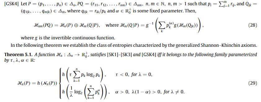
Entropy composability
and group entropies
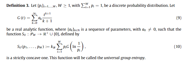
Entropy composability
and group entropies
Entropy and scaling
We have been mentioning the issue of extensivity before
Let us see how the multiplicity and entropy scales with size \(N\)
This allows us to introduce a classification of entropies
How the sample space changes when we rescale its size \( N \mapsto \lambda N \)?
The ratio behaves like \(\frac{W(\lambda N)}{W(N)} \sim \lambda^{c_0} \) for \(N \rightarrow \infty\)
the exponent can be extracted by \(\frac{d}{d\lambda}|_{\lambda=1}\): \(c_0 = \lim_{\rightarrow \infty} \frac{N W'(N)}{W(N)}\)
For the leading term we have \(W(N) \sim N^{c_0}\).
Is it only possible scaling? We have \( \frac{W(\lambda N)}{W(N)} \frac{N^{c_0}}{(\lambda N)^{c_0}} \sim 1 \)
Let us use the other rescaling \( N \mapsto N^\lambda \)
The we get that \(\frac{W(N^\lambda)}{W(N)} \frac{N^{c_0}}{N^{\lambda c_0}} \sim \lambda^{c_1}\)
First correction is \(W(N) \sim N^{c_0} (\log N)^{c_1}\)
It is the same scaling like for \((c,d)\)-entropy
Can we go further?
Multiplicity scaling
-
We define the set of rescalings \(r_\lambda^{(n)}(x) := \exp^{(n)}(\lambda \log^{(n)}(x) \) )
- \( f^{(n)}(x) = \underbrace{f(f(\dots(f(x))\dots))}_{n \ times}\)
- \(r_\lambda^{(0)}(x) = \lambda x\), \(r_\lambda^{(1)}(x) = x^\lambda\), \(r_\lambda^{(2)}(x) = e^{\log(x)^\lambda} \), ...
- They form a group: \(r_\lambda^{(n)} \left(r_{\lambda'}^{(n)}\right) = r_{\lambda \lambda'}^{(n)} \), \( \left(r_\lambda^{(n)}\right)^{-1} = r_{1/\lambda}^{(n)} \), \(r_1^{(n)}(x) = x\)
-
We repeat the procedure: \(\frac{W(N^\lambda)}{W(N)} \frac{N^{c_0} (\log N)^{c_1} }{N^{\lambda c_0} (\log N^\lambda)^{c_1}} \sim 1\),
- We take \(N \mapsto r_\lambda^{(2)}(N)\)
- \(\frac{W(r_\lambda^{(2)}(N))}{W(N)} \frac{N^{c_0} (\log N)^{c_1} }{r_\lambda^{(2)}(N)^{c_0} (\log r_\lambda^{(2)}(N))^{c_1}} \sim \lambda^{c_2}\),
- Second correction is \(W(N) \sim N^{c_0} (\log N)^{c_1} (\log \log N)^{c_2}\)
Multiplicity scaling
- General correction \( \frac{W(r_\lambda^{(k)}(N))}{W(N)} \prod_{j=0}^{k-1} \left(\frac{\log^{(j)} N}{\log^{(j)}(r_\lambda^{(k)}(N))}\right)^{c_j} \sim \lambda^{\bf c_k}\)
- Possible issue: what if \(c_0 = +\infty\)? \(W(N)\) grows faster than any \(N^\alpha\)
- We replace \(W(N) \mapsto \log W(N)\)
- The leading order scaling is \(\frac{\log W(\lambda N)}{\log W(N)} \sim \lambda^{c_0} \) for \(N \rightarrow \infty\)
- So we have \(W(N) \sim \exp(N^{c_0})\)
- If this is not enough, we replace \(W(N) \mapsto \log^{(l)} W(N)\) so that we get finite \(c_0\)
- General expansion of \(W(N)\) is $$W(N) \sim \exp^{(l)} \left(N^{c_0}(\log N)^{c_1} (\log \log N)^{c_2} \dots\right) $$
J.K., R.H., S.T. New J. Phys. 20 (2018) 093007
Multiplicity scaling
Extensive entropy
- We can do the same procedure with entropy \(S(W)\)
- Leading order scaling: \( \frac{S(\lambda W)}{S(W)} \sim \lambda^{d_0}\)
-
First correction \( \frac{S(W^\lambda)}{S(W)} \frac{W^{d_0}}{W^{\lambda d_0}} \sim \lambda^{d_1}\)
- First two scalings correspond to \((c,d)\)-entropy for \(c= 1-d_0\) and \(d = d_1\)
- Scaling expansion of entropy $$S(W) \sim W^{d_0} (\log W)^{d_1} (\log \log W)^{d_2} \dots $$
-
Requirement of extensivity \(S(W(N)) \sim N\) determines the relation between \(c\) and \(d\) :
- \(d_l = 1/c_0\), \(d_{l+k} = - c_k/c_0\) for \(k = 1,2,\dots\)
| Process | S(W) | |||
|---|---|---|---|---|
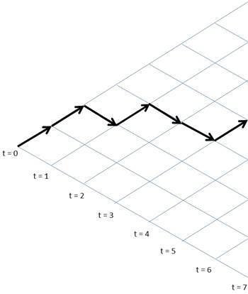
| Random walk |
0 |
1 |
0 |
|
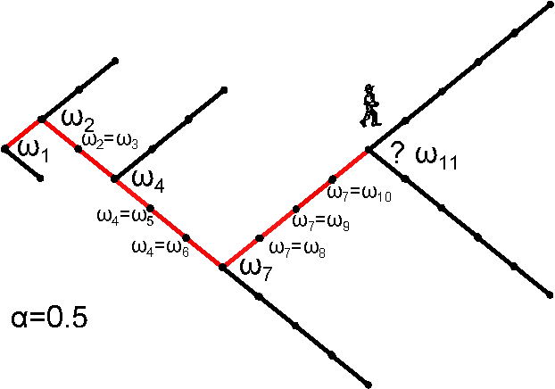
| Aging random walk |
0 |
2 |
0 |
|
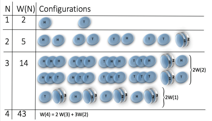
| Magnetic coins * |
0 |
1 |
-1 |
|
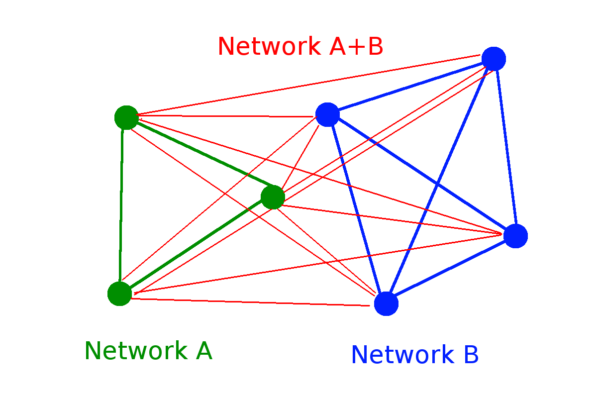
| Random network |
0 |
1/2 |
0 |
|
| Random walk cascade |
0 |
0 |
1 |
\( \log W\)
\( (\log W)^2\)
\( (\log W)^{1/2}\)
\( \log \log W\)
\(d_0\)
\(d_1\)
\(d_2\)
\( \log W/\log \log W\)
* H. Jensen et al. J. Phys. A: Math. Theor. 51 375002
\( W(N) = 2^N\)
\(W(N) \approx 2^{\sqrt{N}/2} \sim 2^{N^{1/2}}\)
\( W(N) \approx N^{N/2} e^{2 \sqrt{N}} \sim e^{N \log N}\)
\(W(N) = 2^{\binom{N}{2}} \sim 2^{N^2}\)
\(W(N) = 2^{2^N}-1 \sim 2^{2^N}\)

Parameter space of \( (c,d) \) entropy
How does it change for one more scaling exponent?
R.H., S.T. EPL 93 (2011) 20006
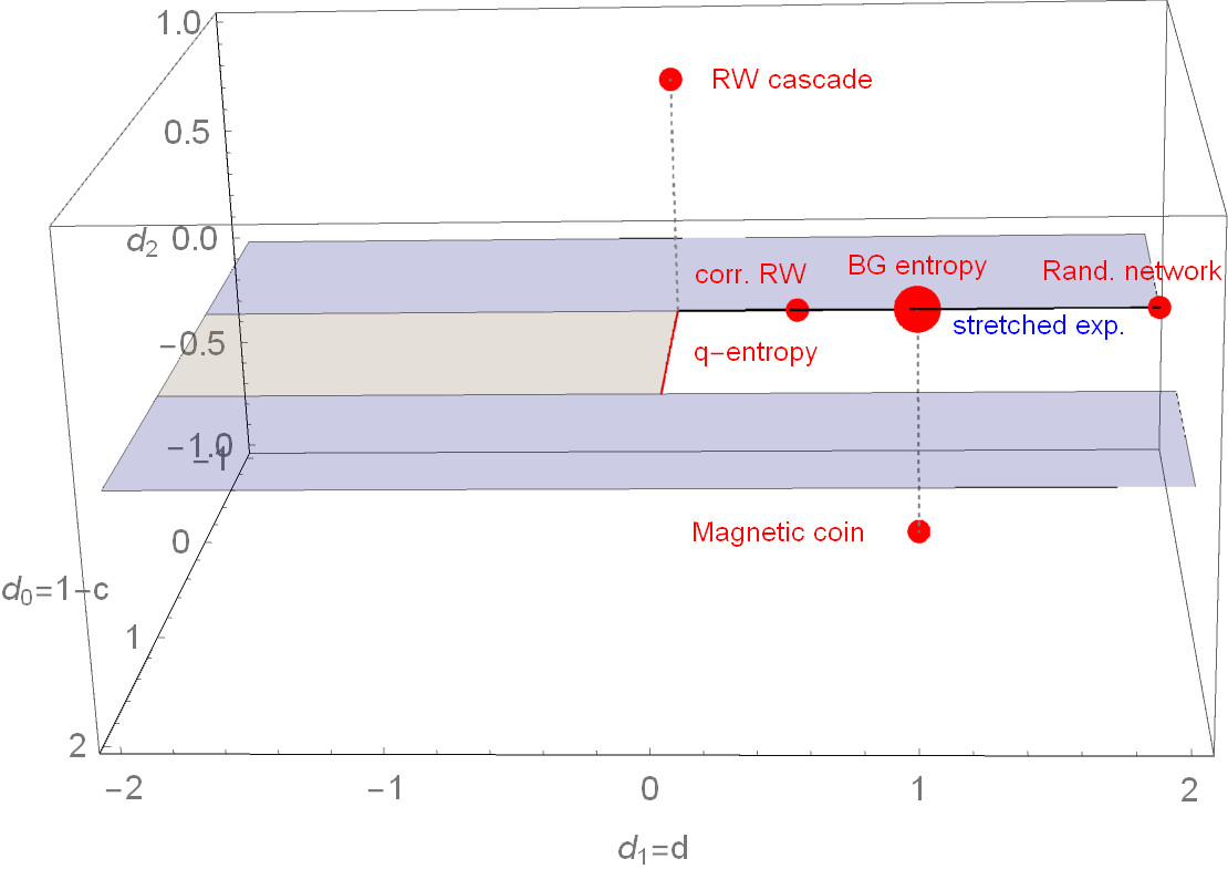
Parameter space of \( (d_0,d_1,d_2) \)-entropy
To fulfill SK axiom 2 (maximality): \(d_l > 0\), to fulfill SK axiom 3 (expandability): \(d_0 < 1\)
- Axiomatization from the Maximum entropy principle point of view
- Principle of maximum entropy is an inference method and it should obey some statistical consistency requirements.
- Shore and Johnson set the consistency requirements:
- Uniqueness.—The result should be unique.
- Permutation invariance.—The permutation of states should not matter.
- Subset independence.—It should not matter whether one treats disjoint subsets of system states in terms of separate conditional distributions or in terms of the full distribution.
- System independence.—It should not matter whether one accounts for independent constraints related to disjoint subsystems separately in terms of marginal distributions or in terms of full-system constraints and joint distribution.
- Maximality.—In absence of any prior information the uniform distribution should be the solution.
Shore-Johnson axioms
P.J., J.K. Phys. Rev. Lett. 122 (2019), 120601
History & Controversy of Shore-Johnson axioms
J. E. Shore, R. W. Johnson. Axiomatic derivation of the principle of maximum entropy and the principle of minimum cross-entropy. IEEE Trans. Inf. Theor. 26(1) (1980), 26. - only Shannon
J. Uffink, Can the Maximum Entropy Principle be Explained as a Consistency Requirement? Stud. Hist. Phil. Mod. Phys. 26(3), (1995), 223. - larger class of entropies including Tsallis, Rényi, ..
S. Pressé, K. Ghosh, J. Lee, K.A. Dill, Nonadditive Entropies Yield Probability Distributions with Biases not Warranted by the Data. Phys. Rev. Lett., 111 (2013), 180604. - only Shannon - not Tsallis
C. Tsallis, Conceptual Inadequacy of the Shore and Johnson Axioms for Wide Classes of Complex Systems. Entropy 17(5), (2015), 2853. - S.-J. axioms are not adequate
S. Pressé K. Ghosh, J. Lee, K.A. Dill, Reply to C. Tsallis’ Conceptual Inadequacy of the Shore and Johnson Axioms for Wide Classes of Complex Systems. Entropy 17(7), (2015), 5043. - S.-J. axioms are adequate
B. Bagci, T. Oikonomou, Rényi entropy yields artificial biases not in the data and incorrect updating due to the finite-size data Phys. Rev. E 99 (2019) 032134 - only Shannon - not Rényi
P. Jizba, J.K. Phys. Rev. Lett. 122 (2019), 120601 - Uffink is correct!
(and the show goes on)
Shannon & Khinchin meet Shore & Johnson
Are the axioms set by theory of information and statistical inference different or can we find some overlap?
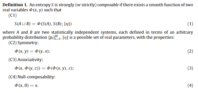
Let us consider the 4th SK axiom
in the form equivalent to composability axiom by P. Tempesta:
4. \(S(A \cup B) = f[f^{-1}(S(A)) \cdot f^{-1}(S(B|A))]\)
\(S(B|A) = S(B)\) if B is independent of A.
Entropies fulfilling SK and SJ: $$S_q^f(P) = f\left[\left(\sum_i p_i^q\right)^{1/(1-q)}\right] = f\left[\exp_q\left( \sum_i p_i \log_q(1/p_i) \right)\right]$$
Phys. Rev. E 101, 042126 (2020)
Non-equilibrium thermodynamics axioms
In ST lecture, you saw that Shannon entropy fulfills the second law of thermodynamics for linear Markov dynamics with detailed balance.
But is it the only possible entropy?
Our axioms are:
1. Linear Markov evolution - \(\dot{p}_m = \sum_n (w_{mn}p_n- w_{nm} p_m)\)
2. Detailed balance - \(w_{mn} p^{st}_n = w_{nm} p^{st}_m\)
3. Second law of thermodynamics: \(\dot{S} = \dot{S}_i + \dot{S}_e\)
where \(\dot{S}_e = \beta Q\), and \(\dot{S}_i \geq 0\) where \(\dot{S}_i = 0 \Leftrightarrow p=p^{st}\)
New J. Phys. 23 (2021) 033049
Then \(S = - \sum_m p_m \log p_m\)
This is a special case of more general result connecting non-linear master equations and generalized entropies
Summary
Foundations of Entropy IV
By Jan Korbel


