Thermodynamics

of structure-forming systems

in collaboration with

Simon D. Lindner   Tuan Pham    Rudolf Hanel     Stefan Thurner 

CSH Workshop Stochastic dynamics for complex systems 

Slides available at: https://slides.com/jankorbel

Thermodynamics

of structure-forming systems

in collaboration with

Simon D. Lindner    Tuan Pham      Rudolf Hanel     Stefan Thurner 

based on a recently published paper: Nat. Comm. 12 (2021) 1127

Slides available at: https://slides.com/jankorbel

Workshop title: Stochastic dynamics for complex systems 

Talk title: thermodynamics of structure-forming systems

     (mostly thermoSTATISTICS)

I hope we will find a common language!                                             

Little warning!

• Historical review of thermodynamics

• Main results of stochastic thermodynamics

• Thermodynamics of structure-forming systems

• Applications to formation of social groups

Outline

Thermodynamics

Microscopic systems

Classical mechanics (QM,...)

Mesoscopic systems

Stochastic thermodynamics

Macroscopic systems

Thermodynamics

Stochastic Thermodynamics is a thermodynamic theory
for mesoscopic, non-equilibrium physical systems
interacting with equilibrium thermal (and/or chemical)
reservoirs

Historical review  of thermodynamics

History

Equilibrium thermodynamics (19 th century)

- Maxwell, Boltzman, Planck, Claussius, Gibbs...

- Macroscopic systems (\(N \rightarrow \infty\)) in equilibrium (no time dependence of measurable quantities - thermoSTATICS)

-  General structure of thermodynamics

• Laws of thermodynamics (general)
• Response coefficients (system-specific)                               

- Applications: engines, refridgerators, air-condition,... 

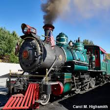
efficiency \(\leq 1-\frac{T_2}{T_1}\)

Heat engine: Carnot cycle

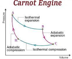
Car engines: 30-50%

History

Laws of thermodynamics

Zeroth law:

Temperature can be measured. $$T_A = T_B \quad \mathrm{if} \quad A \ \mathrm{and} \ B \ \mathrm{are} \ \mathrm{in} \ \mathrm{equilibrium}.$$

First law (Claussius 1850, Helmholtz 1847):

Energy is conserved.
$${\color{aqua} d}U = {\color{orange} \delta} Q - {\color{orange} \delta} W$$ Second law (Carnot 1824, Claussius 1854, Kelvin):

Heat cannot be fully transformed into work. $${ \color{aqua} d} S \geq \frac{{\color{orange} \delta} Q}{T}$$ Third law: We cannot bring the system into the absolute zero
temperature in a finite number of steps. $$ \lim_{T \rightarrow 0} S(T) = 0$$

History

Local equilibrium thermodynamics (1st half of 20th cent.)

- Onsager, Rayleigh...

- Systems close to equilibrium - linear response theory

-  Local equilibrium: subsystems a,b,c are each in equilibrium  

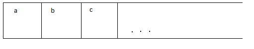
Total entropy \(S \approx S^a + S^b + S^c + \dots\)

Entropy production \(\sigma^a = \frac{d S^a}{d t} = \sum_i Y_i^a J_i^a \)

\(Y_i^a\) - thermodynamic forces; \(J_i^a\) - thermodynamic currents

4th Law of thermodynamics (Onsager 1931): \( \sigma = \sum_{ij} L_{ij} \Gamma_i \Gamma_j\)

 \(\Gamma_i = Y_i^a - Y_i^b \) - afinity, \(L_{ij}\) - symmetric

History and now

Stochastic thermodynamics (90s of 20th century - present)

- Evans, Jarzynski, Crooks, Seifert, van den Broek,....

- Mesoscopic systems far from equilibrium 

- Combines stochastic calculus and non-equilibrium thermodynamics

- Main results: Trajectory thermodynamics, Fluctuation theorems, Thermodynamic uncertainty relations, Speed limit theorems,...

- Applications: colloidal particles and soft matter, biochemistry, molecular motors

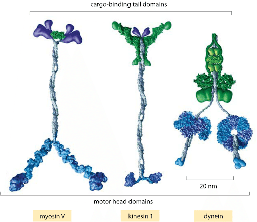
Molecular motor: myosin walking on actin filament

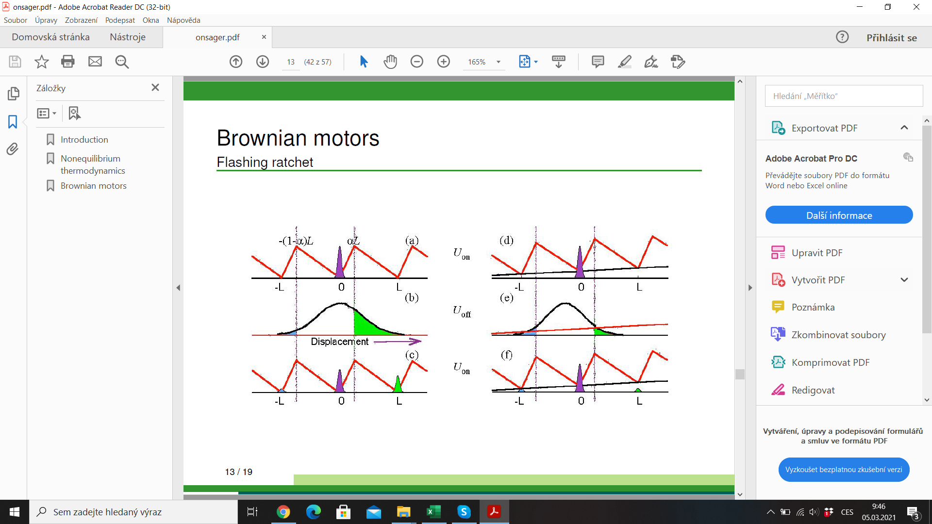
efficiency \(\lesssim 1\)

Main results of stochastic thermodynamics

Stochastic thermodynamics

1.) Consider linear Markov (= memoryless) with distribution \(p_i(t)\).

Its evolution is described by master equation

$$ \dot{p}_i(t) = \sum_{j} [w_{ij} p_{j}(t) - w_{ji} p_i(t) ]$$

\(w_{ij}\) is transition rate. 

2.) Entropy of the system - Shannon entropy  \(S(P) = - \sum_i p_i \log p_i\). Equilibrium distribution is obtained by maximization of \(S(P)\) under the constraint of average energy \( U(P) = \sum_i p_i \epsilon_i \)

$$ p_i^{eq} = \frac{1}{Z} \exp(- \beta \epsilon_i) \quad \mathrm{where} \ \beta=\frac{1}{k_B T}, Z = \sum_j \exp(-\beta \epsilon_j)$$

Stochastic thermodynamics

3.) Detailed balance - stationary state (\(\dot{p}_i = 0\) ) coincides with the equilibrium state (\(p_i^{eq}\)). We obtain

$$\frac{w_{ij}}{w_{ji}} = \frac{p_i^{eq}}{p_j^{eq}} = e^{\beta(\epsilon_j - \epsilon_i)}$$

4.) Second law of thermodynamics: 

$$\dot{S} = - \sum_i \dot{p}_i \log p_i = \frac{1}{2} \sum_{ij} (w_{ij} p_j - w_{ji} p_i) \log \frac{p_j}{p_i}$$

$$ =\underbrace{\frac{1}{2} \sum_{ij} (w_{ij} p_j - w_{ji} p_i) \log \frac{w_{ij} p_j}{w_{ji} p_i}}_{\dot{S}_i} + \underbrace{\frac{1}{2} \sum_{ij} (w_{ij} p_j - w_{ji} p_i) \log \frac{w_{ji}}{w_{ij}}}_{\dot{S}_e}$$

\( \dot{S}_i \geq 0 \) - entropy production rate (2nd law of TD)

\(\dot{S}_e = \beta \dot{Q}\) entropy flow rate

Stochastic thermodynamics

5.) Trajectory thermodynamics - consider stochastic trajectory

\(x(t)= (x_0,t_0;x_1,t_1;\dots)\). Energy \(E_x = E_x(\lambda(t))\), \(\lambda(t)\) - control protocol

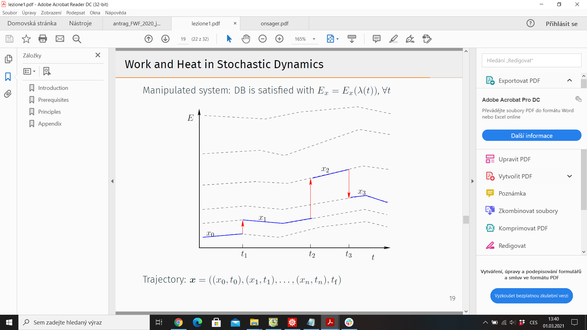
Probability of observing \( x(t)\): \(\mathcal{P}(x(t)\))

Time reversal \(\tilde{x}(t) = x(T-t)\)

Reversed protocol \(\tilde{\lambda}(t) = \lambda(T-t)\)

Probability of observing reversed trajectory under reversed protocol \(\tilde{\mathcal{P}}(\tilde{x}(t))\)

Stochastic thermodynamics

6.) Fluctuation theorems

Trajectory entropy: \(s(t) = - \log p_x(t)\)

Trajectory 2nd law \(\Delta s = \Delta s_i + \Delta s_e\)

Relation to the trajectory probabilities

$$\log \frac{\mathcal{P}(x(t))}{\tilde{\mathcal{P}}(\tilde{x}(t))} = \Delta s_i$$

Detailed fluctuation theorem

$$\frac{P(\Delta s_i)}{\tilde{P}(-\Delta s_i)} = e^{\Delta s_i}$$

Integrated fluctuation theorem $$ \langle e^{- \Delta s_i} \rangle = 1 \quad \Rightarrow \langle \Delta s_i \rangle = \Delta S_i \geq 0$$

Thermodynamics of structure-forming systems

Motivation

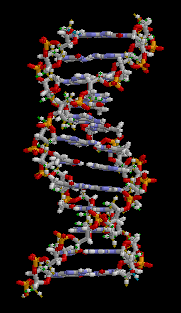
• Many systems form structures: molecules of atoms, clusters of colloidal particles, (bio)polymers or micelles
• We study the thermodynamics of structure-forming systems
• For small systems, we get a correction to Shannon entropy
• We apply the results to several physical systems
• We derive fluctuation theorems for structure-forming systems

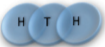
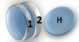
Toy model - magnetic coin model

We consider a coin with two states: head             and tail

The coins are magnetic and can stick together 

How many states we get for N coins?

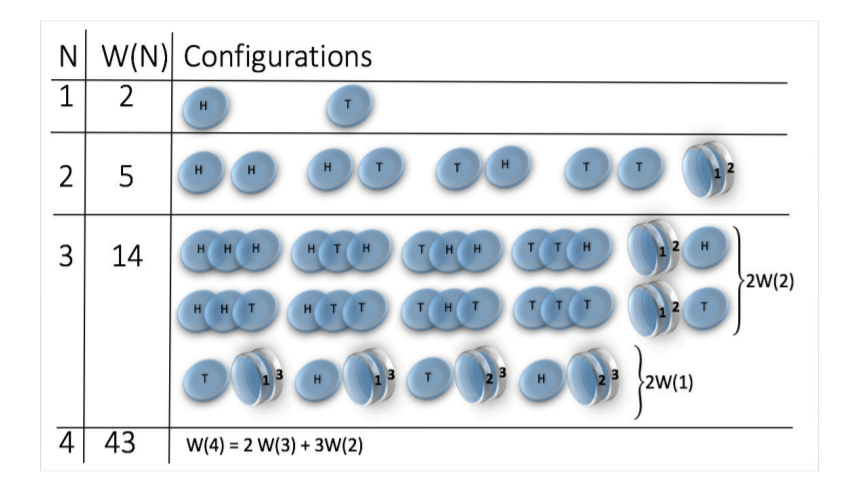
\(W(N) \sim N^N\)

(non-magnetic coins \(W(N) = 2^N\))

picture taken from: H. J. Jensen et al 2018 J. Phys. A: Math. Theor. 51 375002

Multiplicity and entropy

of structure-forming systems

Boltzmann entropy formula: \(S(n_i) = k_B \log W(n_i)\) 

where \(W\) is multiplicity

(number of microstates corresponding to a mesostate \(n_i\))

Microstate: state of each particle

       if more particles are bound to a molecule, then state of each molecule

Mesostate: how many particles and/or molecules are in given state

Example: magnetic coin model: 3 coins, magnetic

                 microstates                       mesostate                 multiplicity

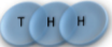
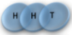
2 x           1x

1 x          1x

3

3

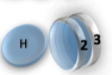
How to calculate a multiplicity?

1. Consider a mesostate
2. Make all permutations of particles
3. Some microstates are overrepresented - calculate how many permutations belong to the same microstate

Examples

2 x           1x

1 x          1x

1    1   2   2    3   3

2   3   1   3    1    2

3   2   3   1    2    1

1    1   2   2    3   3

2   3   1   3    1    2

3   2   3   1    2    1

= (1,2,3) , (2,1,3)

= (1,3,2) , (3,1,2)

= (2,3,1) , (3,2,1)

= (1,2,3) , (1,3,2)

= (2,1,3) , (2,3,1)

= (3,1,2) , (3,2,1)

General formula for multiplicity

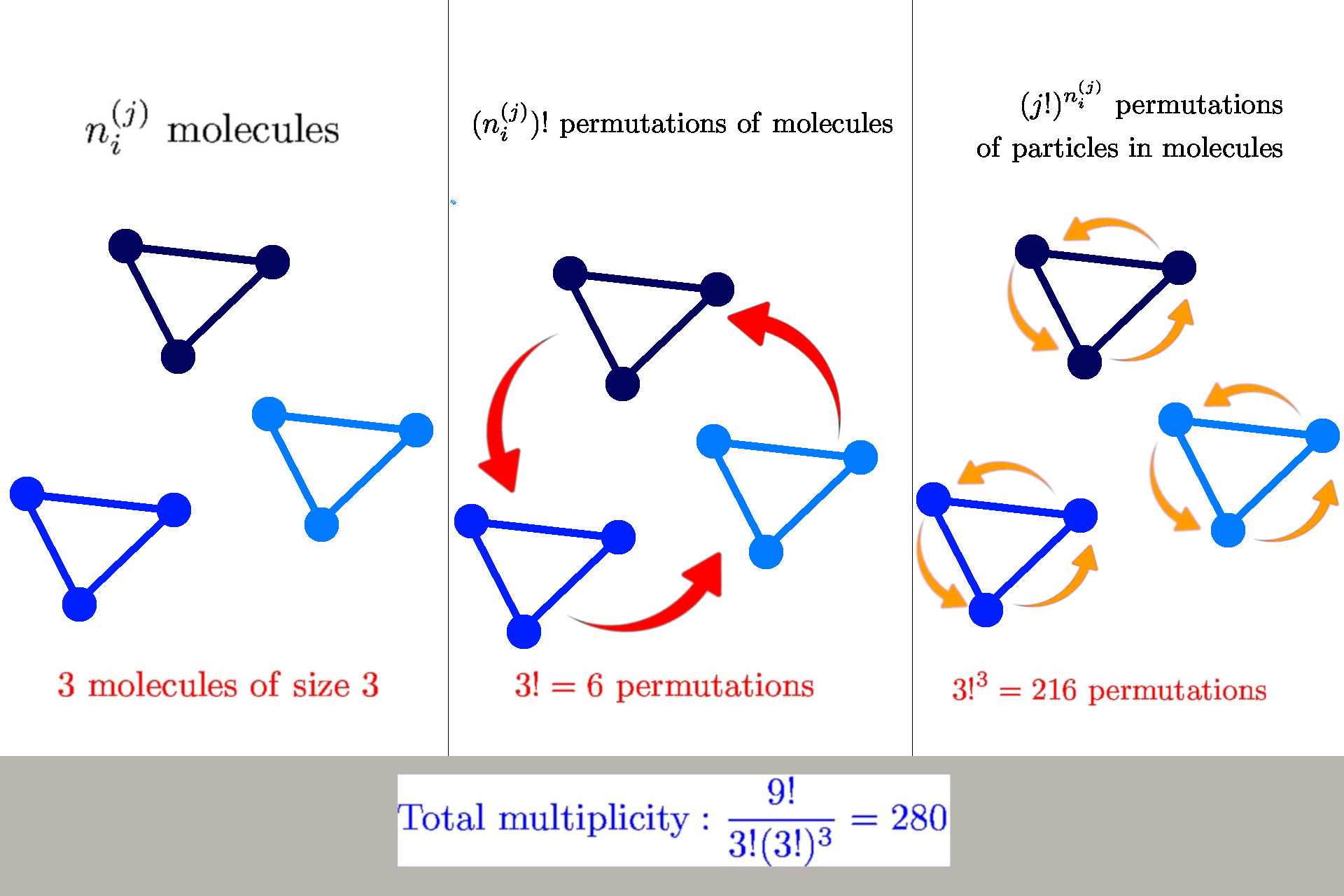
General formula: \(W(n_i^{(j)}) = \frac{n!}{\prod_{ij} n_i^{(j)}!  {\color{aqua} (j!)^{n_i^{(j)}}}}\)  

we have \(n_i^{(j)}\) molecules of size \(j\) in a state \(s_i^{(j)}\)

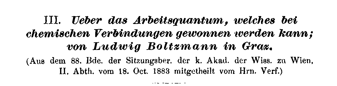
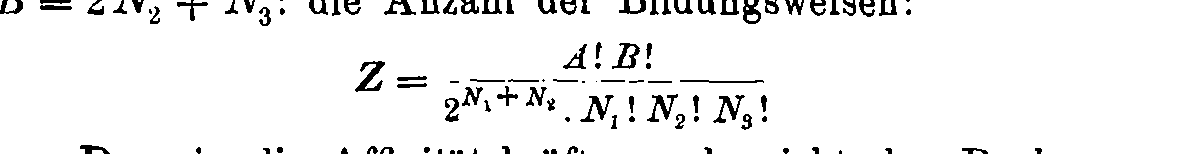
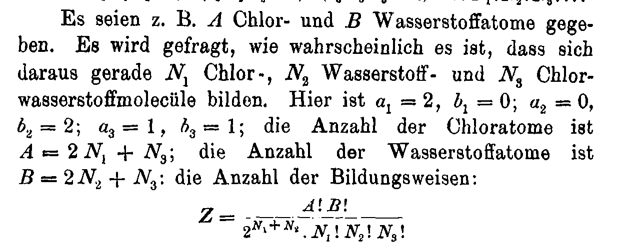
Boltzmann's 1884 paper

Boltzmann's gravestone at Vienna Zentralfriedhof

\( S = k \cdot \log W\)

Entropy of structure-forming systems

$$ S =  \log W \approx n \log n - \sum_{ij} \left(n_i^{(j)} \log n_i^{(j)} - n_i^{(j)} + {\color{aqua} n_i^{(j)} \log j!}\right)$$

Introduce "probabilities" \(\wp_i^{(j)} = n_i^{(j)}/n\)

$$\mathcal{S} = S/n = - \sum_{ij} \wp_i^{(j)} (\log \wp_i^{(j)} {\color{aqua}- 1}) {\color{aqua}- \sum_{ij} \wp_i^{(j)}\log  \frac{j!}{n^{j-1}}}$$

Finite interaction range: concentration \(c = n/b\) 

$$\mathcal{S} = S/n = - \sum_{ij} \wp_i^{(j)} (\log \wp_i^{(j)} {\color{aqua}- 1}) {\color{aqua}- \sum_{ij} \wp_i^{(j)}\log  \frac{j!}{{\color{orange}c^{j-1}}}}$$

Equilibrium distribution:

$$\hat{\wp}_i^{(j)} = \frac{c^{j-1}}{j!} \exp(-\alpha j - \beta \epsilon_i^{(j)})$$

normalization by solving

\(\sum_{ij} j \wp_i^{(j)} = \sum_{ij} \frac{c^{j-1}}{(j-1)!} e^{-{\color{aqua} \alpha} j - \beta \epsilon_i^{(j)}} = 1\) for \({\color{aqua} \alpha}\)

Entropy of structure-forming systems

Main properties:

• The entropy fulfills Shannon Khinchin axioms 1,3,4 but does not fulfill axiom SK 2 (it is not maximized by uniform distribution)
• The entropy fulfills Lieb-Yngvason axioms (it is additive, and it is extensive for \(c=const\) )
• The entropy fulfills Shore-Johnson axioms 1,3,4 but does not fulfill axioms SJ 2 (permutation/coordinate invariance)
• The entropy fulfills Tempesta group-composability axiom but is not symmetric in its arguments
• The scaling exponents according to Hanel-Thurner axioms are                           \(c=0,d=1\), the same as for Shannon entropy

\( \Rightarrow\) The entropy satisfies all common axiomatic schemes but it is not symmetric in probabilities

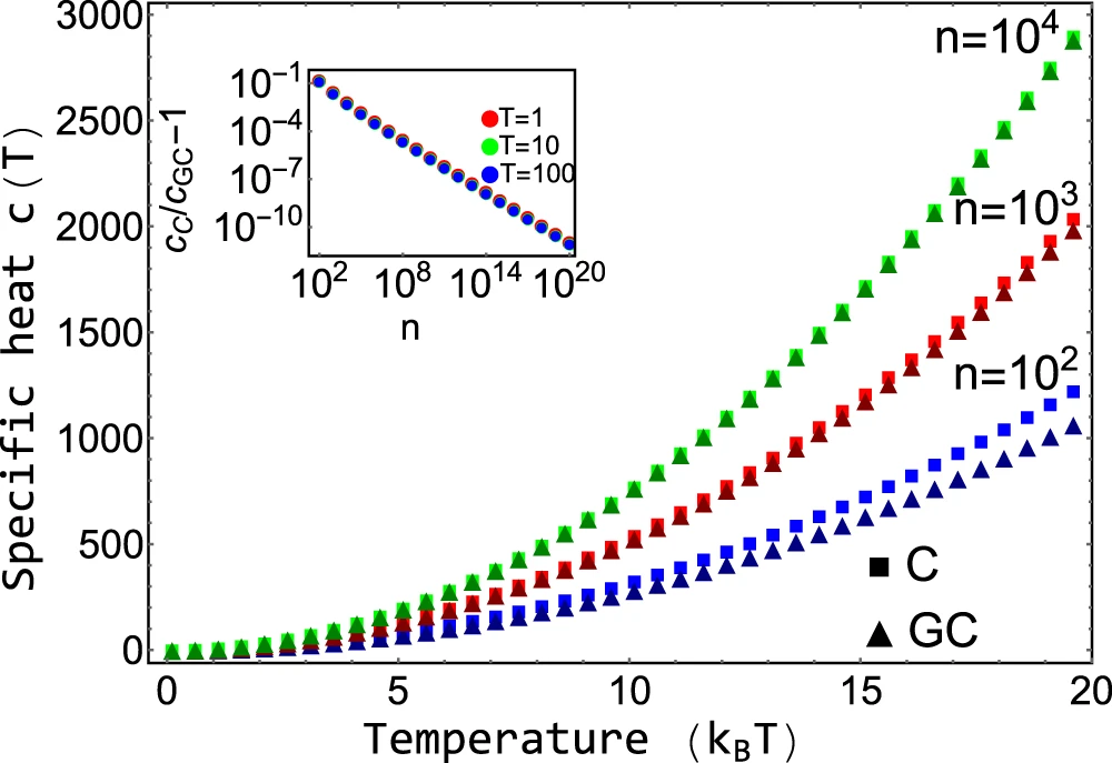
Comparison with Grand-canonical ensemble

Stochastic thermodynamics of structure-forming systems

1. Linear Markov (= memoryless) with distribution \(\wp_i(t)\).

Its evolution is described by master equation

$$ \dot{\wp}_i(t) = \sum_{j} [w_{ij} \wp_{j}(t) - w_{ji} \wp_i(t) ]$$

\(w_{ij}\) is transition rate. 

2. Detailed balance

Assumptions

Stochastic thermodynamics of structure-forming systems

Results

1. Second law of thermodynamics for non-equilibrium systems

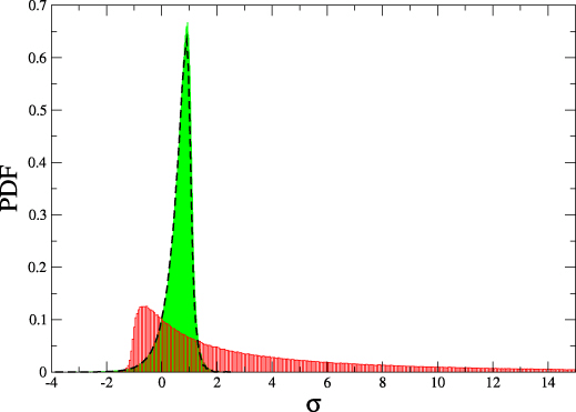
2. Detailed fluctuation theorem for structure forming systems

$$\frac{P(\Delta \sigma)}{\tilde{P}(-\Delta \sigma)} = e^{\Delta \sigma}$$

where  \(\Delta \sigma = \Delta s_i +  {\color{aqua} \log j_0 - \log j_f}\)

\(\Delta s_i\) is the trajectory entropy production

Applications to physics

 Self-assembly of Janus particles

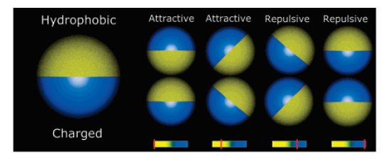
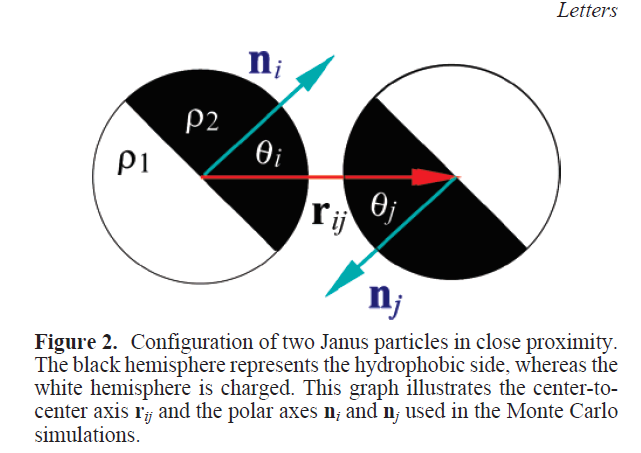
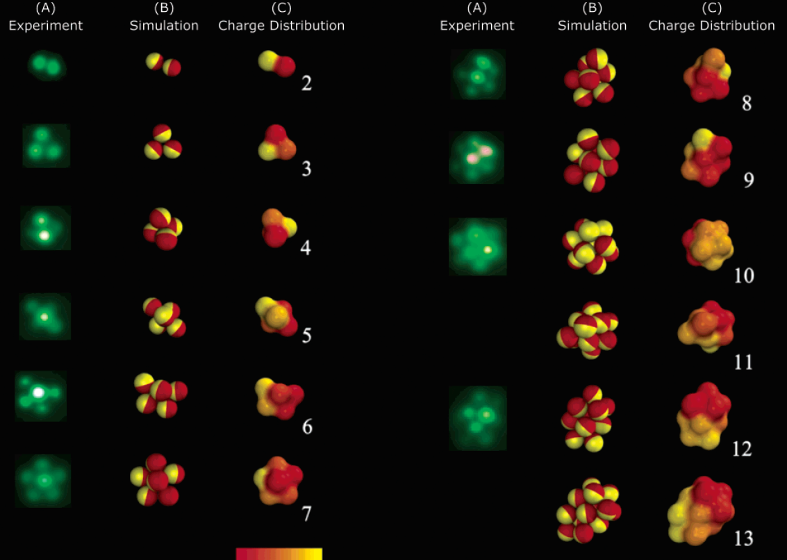
Kern-Frenkel model

Pair-wise potential: \(U^{KF}(r_{ij},n_i,n_j) = u(r_{ij}) \Omega(r_{ij},n_i,n_j) \)

Square-well interaction with hard sphere: 

$$ u(r_{ij}) = \left\{ \begin{array}{rl} \infty, & r_{ij} \leq \sigma \\  - \epsilon, & \sigma < r_{ij} < \sigma + \Delta \\ 0, & r_{ij} > \sigma + \Delta. \end{array} \right.$$

\(\Omega\) decribes orientation of particles:

Particle coverage \(\chi = \sin^2(\theta/2) = \frac{1-\cos{\theta}}{2}\)

Polymers: \(\chi = 0.3\)

Janus particles: \(\chi = 0.5\)

Crystalic structures: \(\chi = 0.6\) (stable lamellar crystals)

$$\Omega(r_{ij},n_i,n_j) = \left\{\begin{array}{rl} -1 & \mathrm{if} \  r_{ij} \cdot n_i > \cos(\theta) \ \mathrm{and} \ r_{ij} \cdot n_j > \cos(\theta)\\ 0 & \mathrm{otherwise} \end{array}  \right.$$

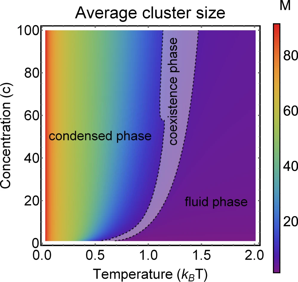
Phase diagram of Janus particles for average cluster size \(M\)

Currie-Weiss model with molecules

(= fully connected Ising model with bound states)

$$ H(s_i) = - \frac{J}{n-1} \sum_{i \neq j, \ free} s_i s_j - h \sum_{j, \ free} s_j $$

Applications to

group formation

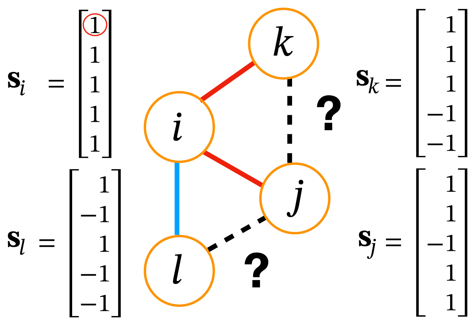
Homophily in social networks

Two individuals are friends if they have more similar opinions

Two individuals are enemies if they have more different opinions

Group formation based on homophily

Hamiltonian of a group \(\mathcal{G}\)

\(H(\mathbf{s}_{i_1},\dots,\mathbf{s}_{i_k}) =  \underbrace{- \phi \, \frac{J}{2} \sum_{ij \in \mathcal{G}} A_{ij} \mathbf{s}_i \cdot \mathbf{s}_j}_{\textcolor{red}{intra-group \ social \ stress}}+ \underbrace{(1-\phi) \frac{J}{2} \sum_{i \in \mathcal{G}, j \notin \mathcal{G}} A_{ij} \mathbf{s}_{i} \cdot \mathbf{s}_j}_{\textcolor{blue}{inter-group \ social \ stress}} \\ \qquad \qquad \qquad \qquad - \underbrace{h \sum_{i \in \mathcal{G}} \mathbf{s}_i \cdot \mathbf{w}}_{external \ field}\)

Group formation based on opinion= self-assembly of spin glass

Group 1

Group 2

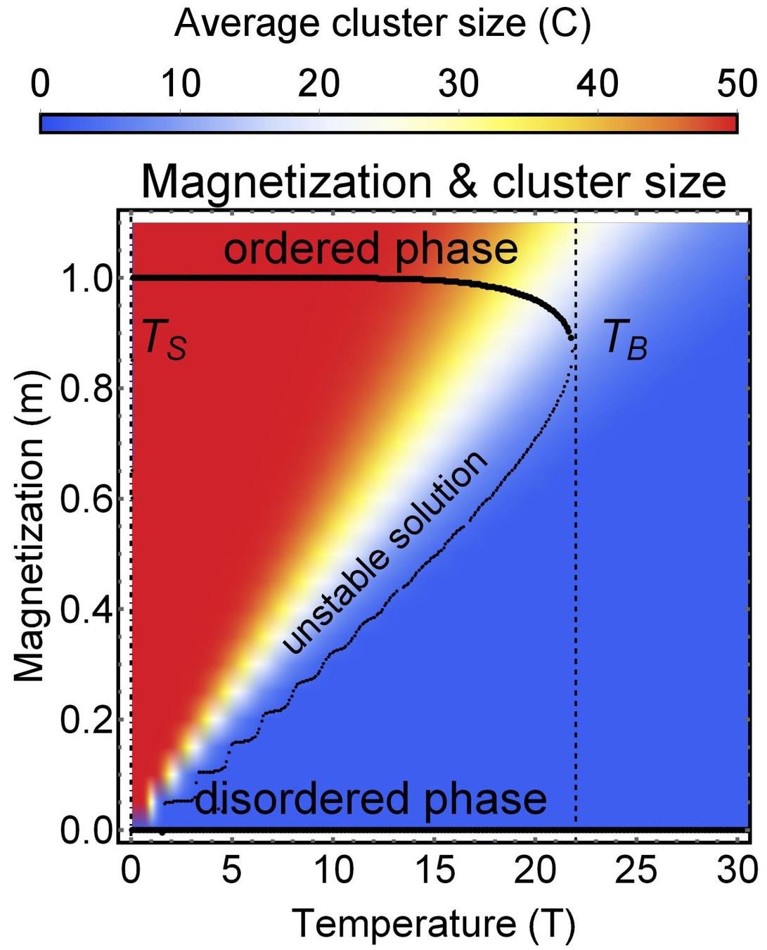
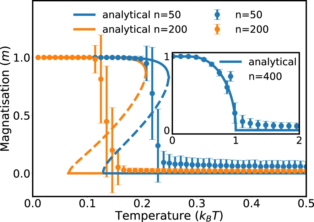
Phase diagram of group size 

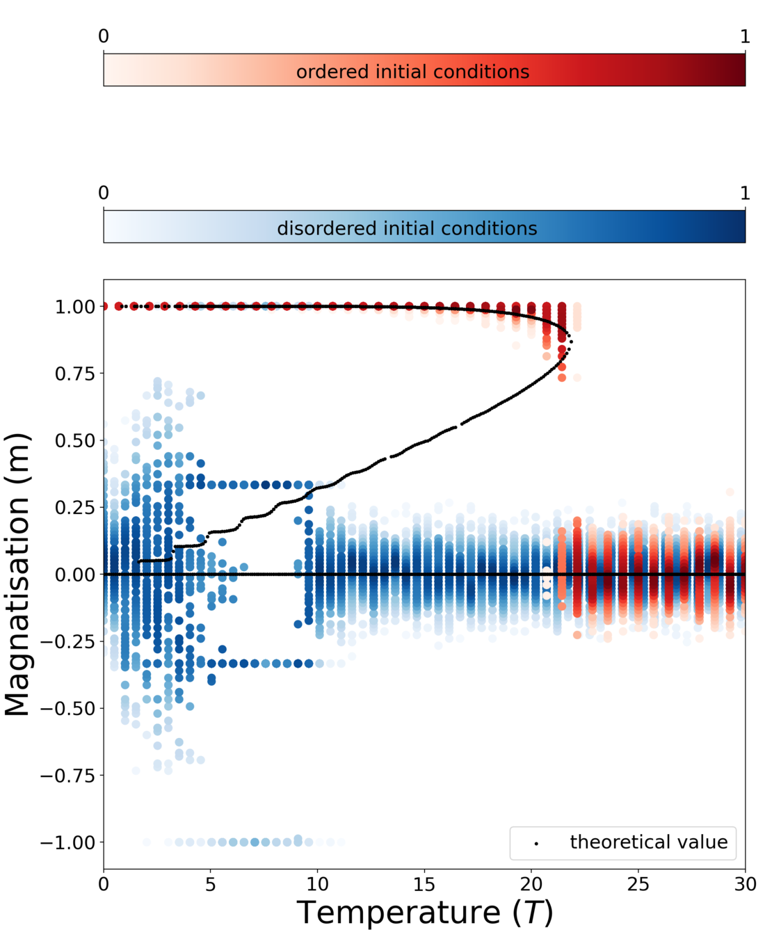
Theory

MC simulation

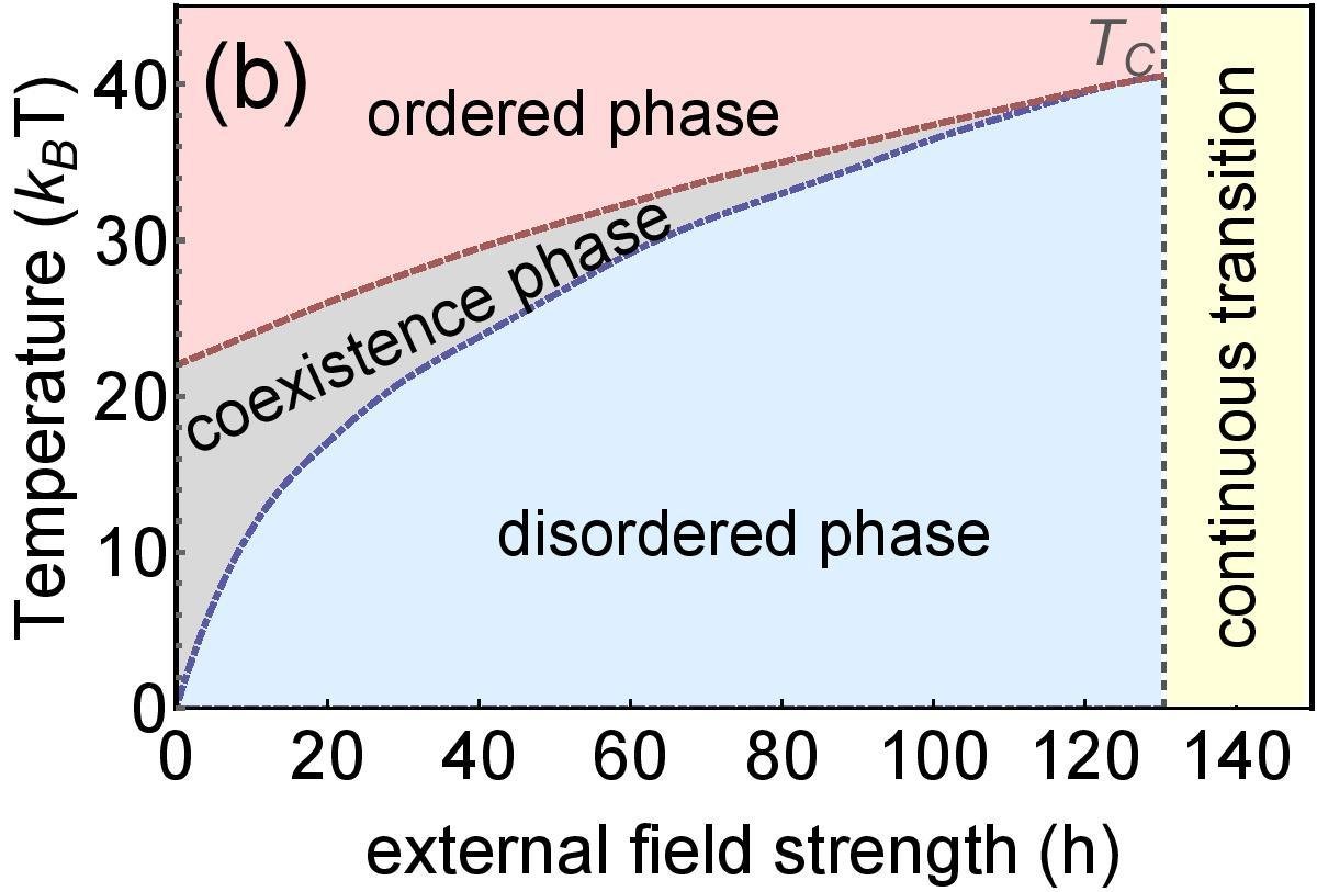
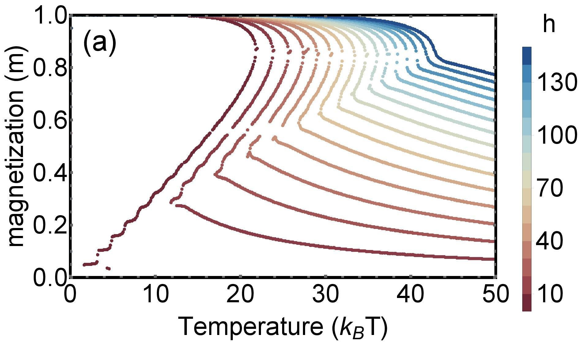
Dependence on external field

Application to real example of a massive online multiplayer game (PARDUS)

Summary

More details in: J. K., S. D. L., R. H. and S. T., Nat. Comm. 12 (2021) 1127