introduction to statistics
Javier Sajuria
UCL - Political Science
Session 2
1 February 2014
review of descriptive statistics
Given the following variables, what are the appropriate measures of central tendency and dispersion?
- A variable indicating allegiance to a political party, where 1 = Conservative, 2 = Labour, 3 = Liberal Democrat and 4 = Another Party
- A variable indicating the difference in the percentage of votes received by Democratic and Republican U.S. Presidential candidates in all elections since World War II
-
A survey measure of interest in politics, where users are asked to indicates their interest on a whole number scale that ranges from 1-10, where 1 = No Interest and 10 = Very Interested
agenda
- What is probability and why is it important?
- Probability distributions
- The normal curve
- Standard deviation units and z-scores
- The sampling distribution of means
- Central Limit Theorem
- Standard Error
additional vocabulary

more practice

what is probability?
- Probability tells us how likely it is that a certain outcome will occur.
- We often do not know probabilities, so we estimate them
- In randomly collected data, however, we can predict with a good amount of certainty, how likely specific outcomes are
- The probability that an observation has a particular outcome is the proportion of times it would occur over a long sequence of observations
-
Since all probabilities are proportions, probabilities are always bound between 0 and 1
probability
-
Think about flipping an unweighted coin
-
In a short sequence of 10 flips, you may get 7 heads and 3 tails, 10 heads and 0 tails, 2 heads and 8 tails
-
In short sequences, the observed probabilities will vary
-
In a long sequence, you should get heads half the time and tails half the time
-
The probability of getting heads over 1000 flips is about .5 and the probability of getting tails is about .5
-
If you flipped an infinite number of times, the probabilities would be (in theory) exactly .5 for both heads and tails
why is probability important?
-
Probability is the key tool that allows us to determine how representative our sample is of the wider population
-
It allow us to say how likely we would be to get the same results from another sample
-
It allows us to make inferences about the population even when we don’t know the true population parameters
probability distribution
-
A probability distribution is like a frequency distribution
-
But rather than simply listing the number of times a value occurs, it tells us the probability of each value occurring, or the proportion of times it occurs
-
So, if we flipped a coin 10 times and 4 times it was heads and 6 times it was tails, a probability distribution would tell us that heads = 0.4 and tails = 0.6
probability distribution
-
If we are given an ordinal set of data, we can work out a probability distribution by hand and look at it graphically
-
We must divide the number of times a response option occurs by the total number of possible observations
-
Do this for each possible response/coding option
-
Added together, the individual response probabilities should total to 1
example probability distribution
Suppose you have randomly sampled 100 countries and measured their level of democracy on a scale from 1 to 5 with 5 being the most democratic and 1 being the least democratic. Your data produces the following frequency distribution:
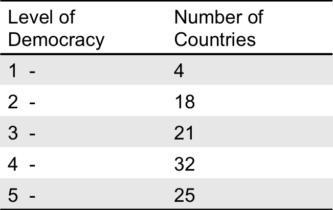
example
We can find the probabilities of each value by dividing the number of occurrences by the total number of observations
So 4/100 = .04
We get the following probability distribution

Represented graphically

probability distributions and continuous data
When we plot probability distributions of continuous data, we get a curve
Theoretically, with continuous data there are an infinite number of values
Consider the example from Agresti and Finlay (pg. 77): amount of time it takes respondents to get to work
In theory, you could break down those times further and further so they eventually form a curved line rather than a bar chart/histogram
continuous
When we look at a probability distribution for continuous data, we are actually trying to find the area under the curve (see A&F, 77)
So if we want to determine what proportion of the population spends an hour or more commuting to work, we would find the area under the curve beginning at 1 hour
continuous
If we plotted our continuous data as a bar chart we’d get something like this
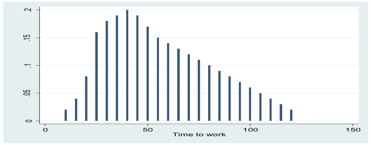
We can imagine a curve being drawn on it
More on probability distributions
Like frequency distributions, probability distributions have means and standard deviations
We can use these values to learn more about our sample compared to the population
So far, we have only looked at sample probability distributions
But there is much more we can know than the simple probability of one event occurring
mean of a probability distribution

the normal curve

the normal curve

the normal curve graphically
the standard normal distribution
-
It is the standard normal distribution helps us make statistical inferences
-
It has the two following properties
- μ = 0
- σ = 1
-
For our purposes, we typically refer to the standard normal distribution
-
But remember, for any mean and corresponding standard deviation, there is a normal curve with those values
The Normal Curve and Standard Deviation UNITS
Last week we found the standard deviations in a few frequency distributions
We can use that number to map a frequency distribution onto a standard normal probability distribution
The reason is that there is a ‘value-based’ standard deviation that correlates with the standard deviation units of the standard normal distribution
Important because standard deviation units can be translated into probabilities
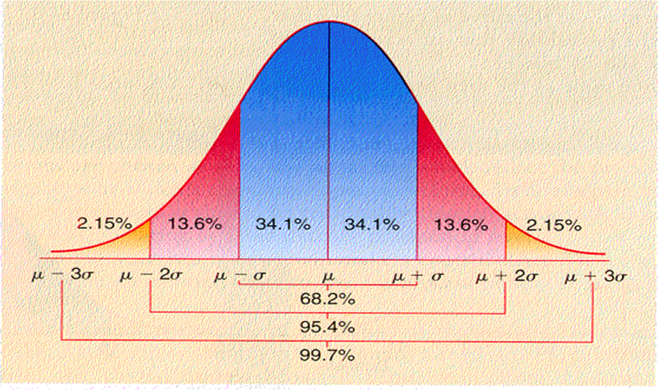
the normal curve and standard deviation units
-
If we look within 1 standard deviation unit (σ) either side of the mean, the normal curve will encompass 68.2% of all possible observations
-
If we look within 2 standard deviation units (2σ) either side of the mean, the normal curve will encompass 95.4% of all possible observations
-
If we look within 3 standard deviation units (3σ) either side of the mean, the normal curve will encompass 99.7% of all possible observations
-
Let’s think about what this means… (no pun intended)
THE NORMAL CURVE AND STANDARD DEVIATION UNITS

This is the graphical representation of the area under the curve
Remember, with continuous data – which a probability distribution is – finding the probability of certain observations means finding the area under the curve
This curve can map onto a distribution in which we have found the mean and the standard deviation (not in sd units)
If we think of the continuous variable IQ score with a mean of 100 and a standard deviation of 18, how would that correspond to the normal curve above?
Remember though, they are measuring slightly different things…the normal curve is a probability distribution and the summary of IQ scores would be a frequency distribution
An Example: Standard Deviation and Standard Deviation Units

some technicalities
-
If we look back
at the normal
curve, we can
see that technically, it is 68.2% and 95.4% that are ±σ and ±2σ, respectively.
- We are especially concerned with the 95.4% If we want to be at exactly 95%, this is technically 1.96 standard deviation units, not 2.

z-scores

z-scores
finding the z-score
Suppose you have a sample of 142 individuals with a mean age of 38 and standard deviation of 14
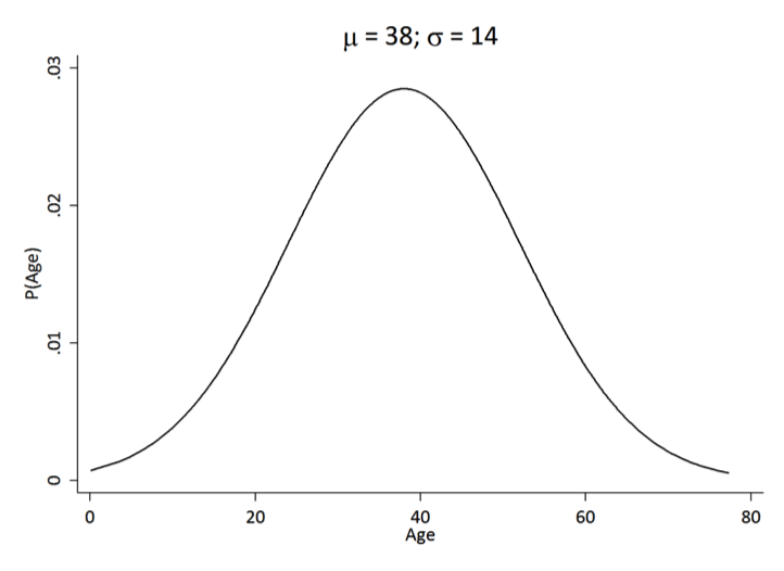
What is the z-score for a 51 year-old?
finding the z-score
z = 51−38/14 = 0.93
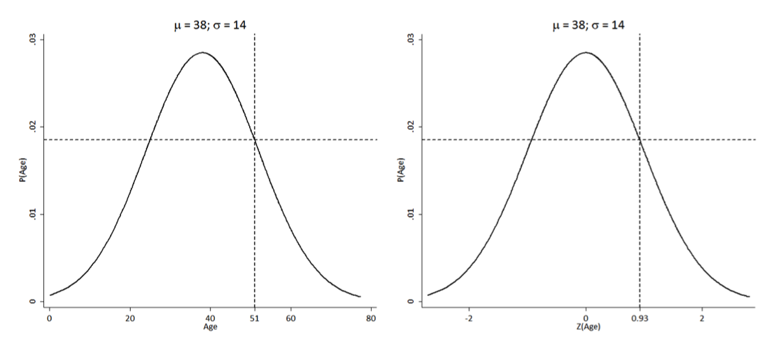
How should we interpret a z-score of 0.93?
How would the z-score change if the standard deviation were 6, instead of 14?
finding the z-score
z = 51−38/6=2.12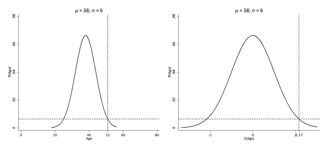
How should we interpret a z-score of 2.12?
sampling distribution of means
-
So, how does the normal curve help us make inferences about the population?
-
Particularly when some variables are not, themselves, normally distributed?
-
Through the sampling distribution of means
-
The sampling distribution of means is the mean of all possible means (mean of means)
-
A sampling distribution of means is always normal
sampling distribution of means
-
Example: Imagine a sample of 3 individuals asked about their favourite ice cream flavour – vanilla or chocolate
-
We could exhaust all possible samples as follows
- (V,V,V) (V,V,C) (V,C,V) (V,C,C)
- (C,C,C) (C,C,V) (C,V,C) (C,V,V)
- Now, we can find the probability of our sample choosing chocolate based on these
-

sampling distribution of means
-
However, our samples are rarely 3 people
-
We can imagine taking samples of 100 in which respondents choose either chocolate or vanilla
-
This gives us 10,000 possible samples…with only 2 choices!
-
If we increase the options to chocolate, vanilla, or strawberry, it gives us 1 million distinct possible samples
-
As our sample size or our response options increase, the number of possible unique samples grows
sampling distribution of means

sampling distribution of means

central limit theorem

standard error

standard error
-
The standard error is the standard deviation of the sampling distribution of means (A&F p. 90)
-
It is sometimes referred to as Random Sampling Error or the Standard Error of the Mean
-
It is denoted:

-
The standard error tells us how much our sample is likely to differ randomly from the population, even when we don’t know the mean of the population
-
It cannot account for systematic error in our data or issues of bias
standard error

standard error
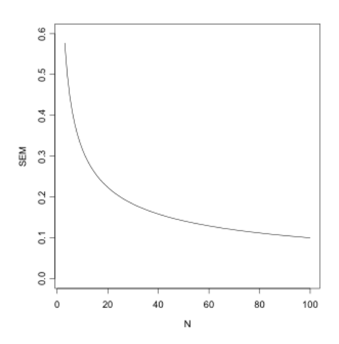
The formula for standard error suggests that as sampling size increases, sampling error decreases
calculating standard error

another example
-
You have surveyed 127 of your classmates to find out the mean number of hours per week they spend writing for their PhDs.
- μ = 22
- σ = 9
-
Find the standard error
-
What if you were able to increase the sample size to 216 and the other statistics remained the same?
-
What if you had only been able to survey 48 of your classmates?
calculations
9/√127 = (9/11.3)
= .80
9/√216 = (9/14.7)
= .61
9/√48 = (9/6.9)
= 1.30
Effect of larger sample size is to decrease estimate of standard error
interpreting the standard error
Like the standard deviation, there is no set value we look for in the standard error
This is because it is based on the units in which the data is measured
However, larger numbers mean more error and smaller numbers mean less
The previous example shows what happens to the standard error as sample sizes increase and decrease
putting it all together
-
To estimate confidence intervals, you must calculate the mean and the standard error
-
To estimate the standard error, you must calculate the standard deviation and the sample size
-
To estimate the standard deviation, you must know the mean, each observation, and the sample size
Seminar Activity
- Activity 1: http://bit.ly/seminar1bbk
- Activity 2 file: http://bit.ly/seminar2bbk
- Activity 3 file: http://bit.ly/seminar3bbk
- Activity 4 file: http://bit.ly/1bhgfPG
introduction to statistics
By Javier Sajuria


