Igusa zeta functions and hyperplane arrangements
How to Navigate:
Spacebar: Forward
Shift + Spacebar: Backward
Escape: Jump around
Arrow keys: Move around
The Igusa zeta function
Let \(f\in \mathbb{Z}[x_1, \dots, x_d]\). For every positive integer \(n\):
- Can we write a formula for \(R(n)\)?
If \(n = p_1^{e_1} \cdots p_{\ell}^{e_{\ell}}\) is the prime factorization of \(n\), then
So we focus on a prime \(p\).
- How does \(R(p_i^{e_i})\) vary as \(i\) varies?
- How does \(R(n)\) grow as \(n\) grows?
- Only finitely many different formulae for the \(R(p^e)\) over all primes \(p\)?
We focus on polynomials equal to product of linear factors.
Leading terms!
Theorem (Igusa 1974).
- The \(R(p^e)\) grow like a polynomial,
- only finitely many different formulae for \(R(p^e)\), and
- there is a finite linear recurrence relation among \(R(p^{e_i})\).
Example.
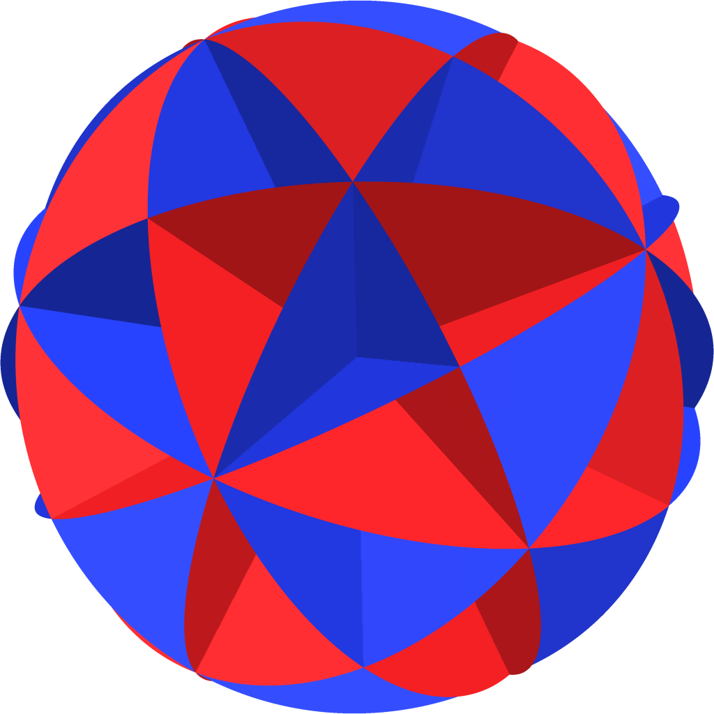
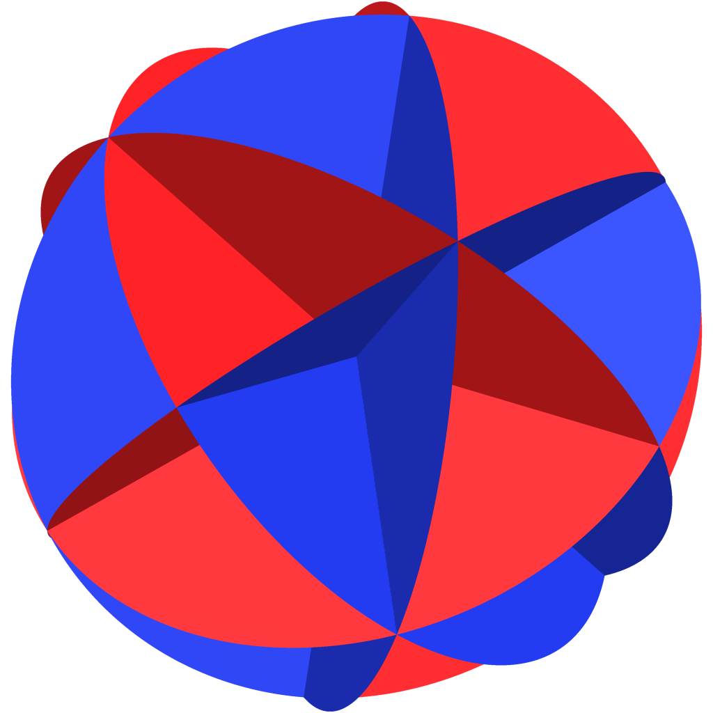
- \(p >2\)
- \(p =2\)
Overview
Understand features of Igusa zeta function with combinatorial & topological tools
flag Hilbert–Poincaré series
Igusa zeta function
combinatorial "coarsening"
Define flag Hilbert–Poincaré series and give substitution.
Hyperplane arrangements
Hyperplane arrangement \(\mathcal{A}\) finite set of hyperplanes in \(K^d\).
Intersection poset: ordered by reverse inclusion
- Bottom element \(\hat{0}\) : the vector space \(K^d\).
- Top element \(\hat{1}\) : the common intersection (if exists).
If \(\hat{1}\in\mathcal{L}(\mathcal{A})\), then \(\mathcal{A}\) is central.

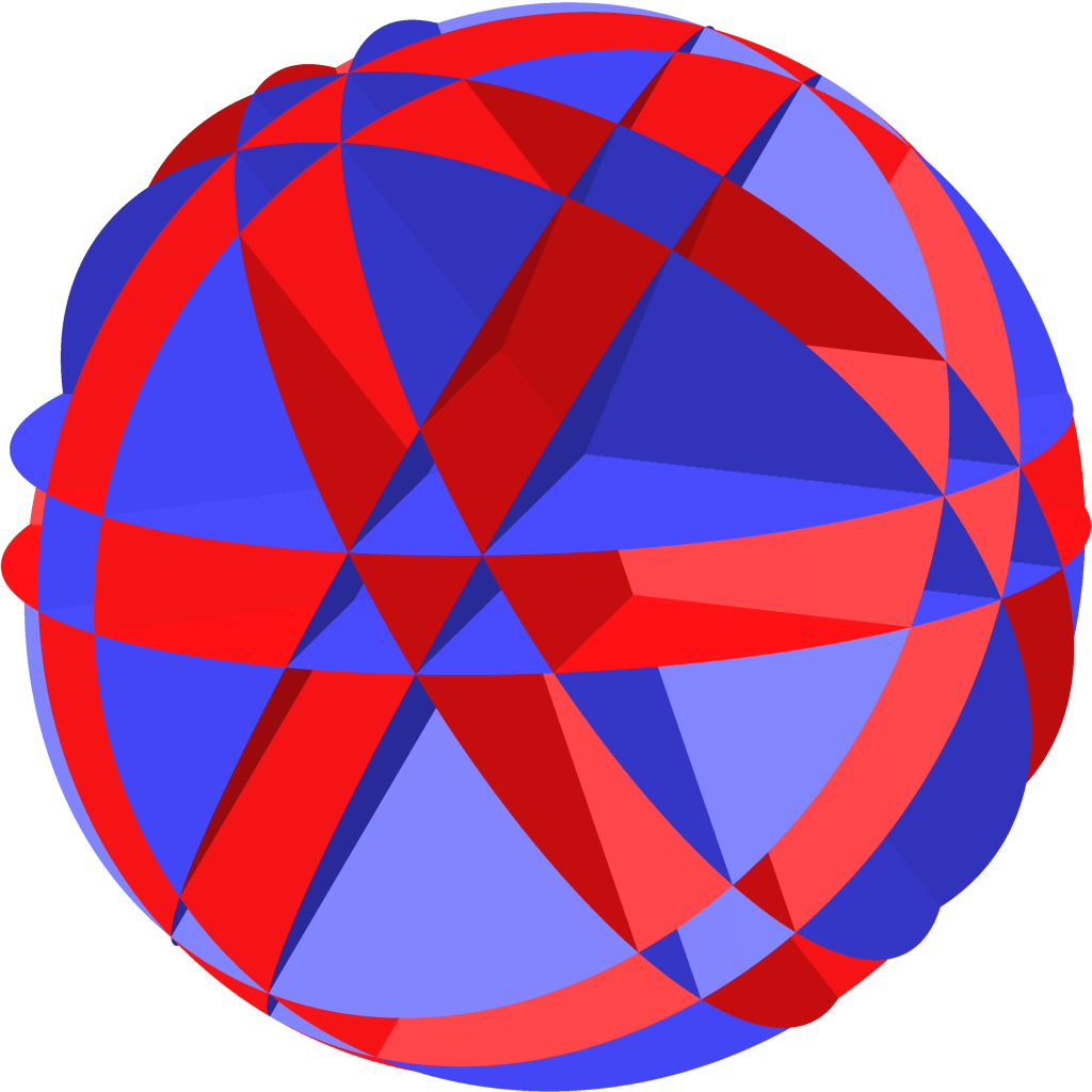
Poincaré polynomial:
Coefficients are Betti numbers.
Example.
\(\mathrm{codim}\)
0
1
2
3
\(\mathcal{L}(\mathsf{A}_3)\)
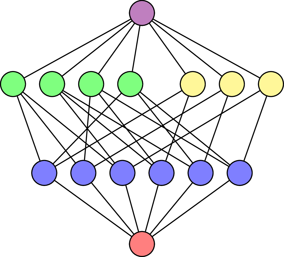
\(\hat{0}\)
\(\hat{1}\)

\(\mathsf{A}_3\)
\(K\!=\!\mathbb{C}\)
Write \(\Delta(\mathcal{L}(\mathcal{A})\setminus \{\hat{0}\})\) for flags of proper subspaces in \(\mathcal{L}(\mathcal{A})\).
For flag \(F = (F_1< \cdots <F_{\ell}) \in \Delta(\mathcal{L}(\mathcal{A})\setminus \{\hat{0}\})\), generalize:
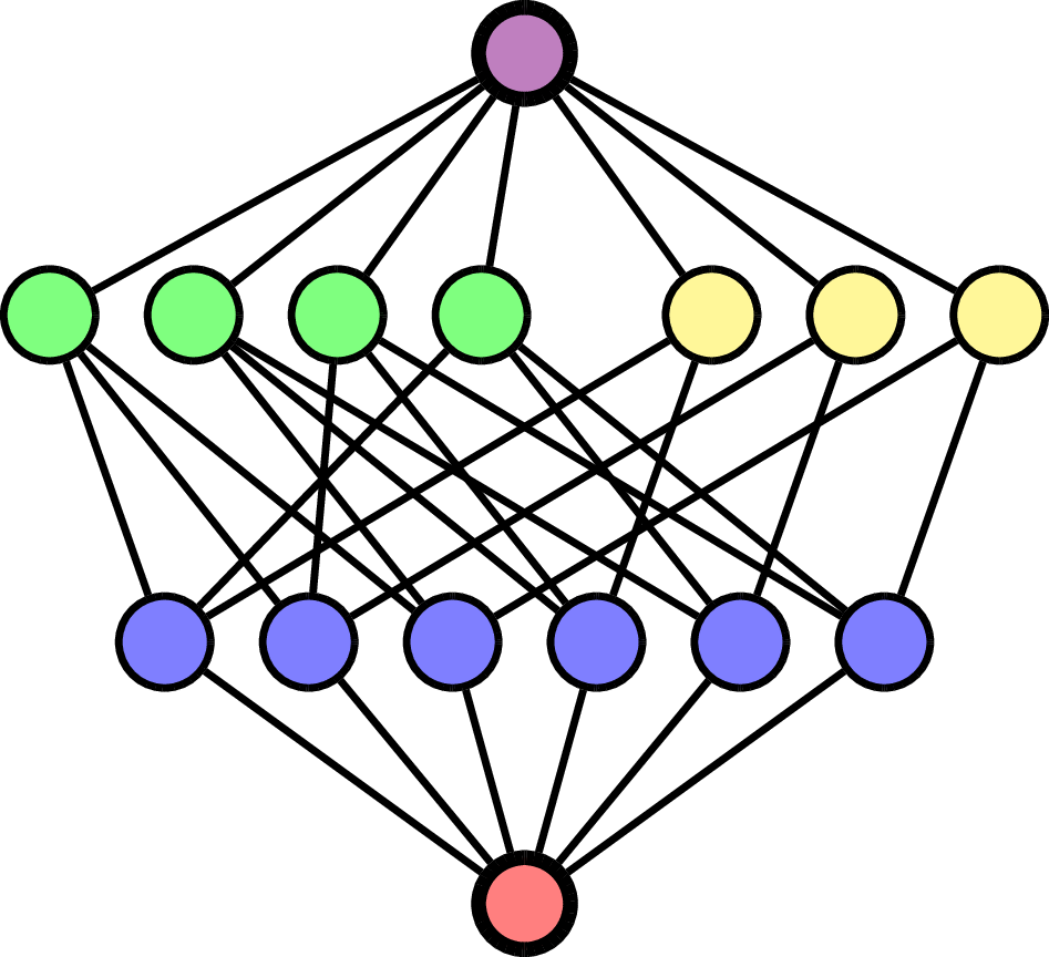
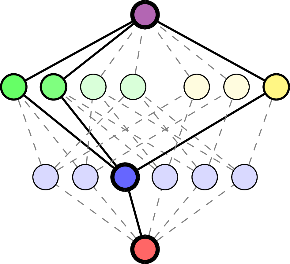
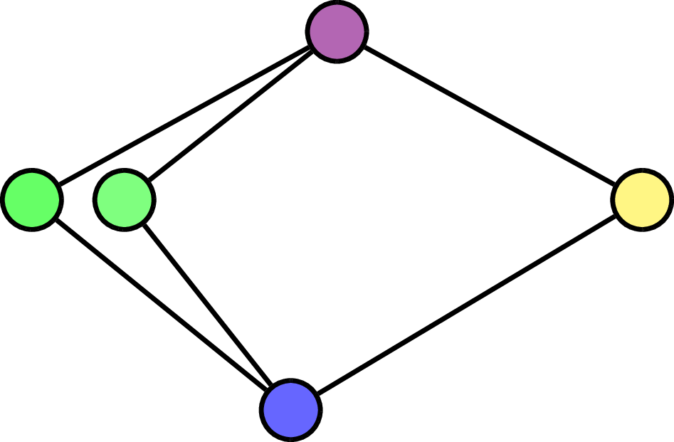
Example.
\(F = (\quad\;)\):




Self reciprocity
The flag Hilbert–Poincaré series:
Idea: \(\mathsf{fHP}_{\mathcal{A}}\) is equivalent to a multivariate \(p\)-adic integral.
Theorem (M., Voll 2024). For \(\mathcal{A}\) defined over field of characteristic \(0\) and central, then
For \(x\in\mathcal{L}(\mathcal{A})\), set
All potential poles come from combinatorial data:
Back to Igusa zeta functions
is the Igusa zeta function associated to \(\mathcal{A}\).
Theorem (M., Voll 2024). If \(\mathcal{A}\) defined over \(\mathbb{Q}\), then for all but finitely many primes \(p\),
Example.
Back to our original data:
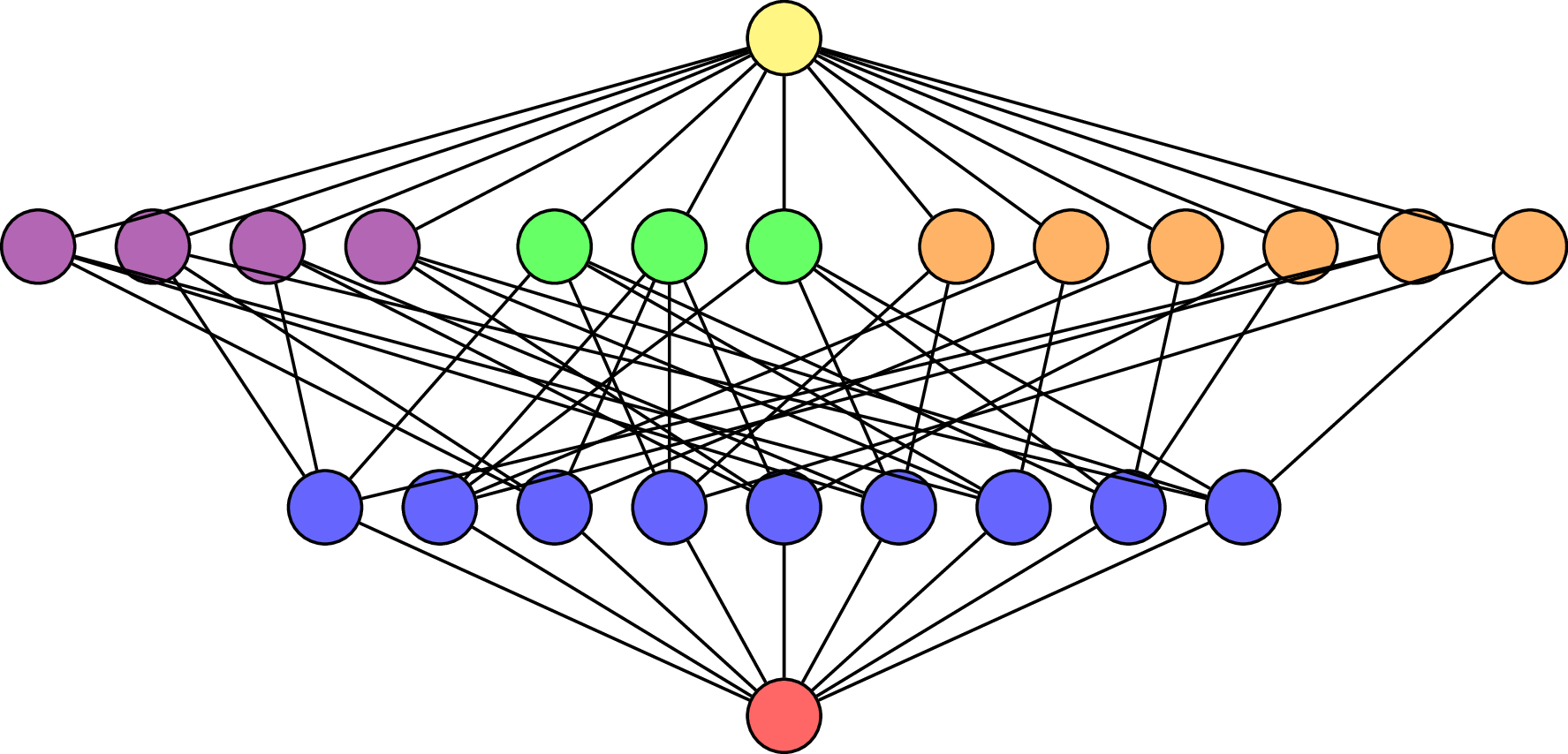
\(\mathcal{L}(\mathsf{B}_3)\)


A different coarsening
Set each \(T_x=T\) — coarse flag Hilbert–Poincaré series:
Nice form:
of \(\mathcal{L}(\mathcal{A})\)
codim of
maximal elt
Corollary. For every hyperplane arrangement \(\mathcal{A}\), the coefficients of \(\mathcal{N}_{\mathcal{A}}(Y, T)\) are non-negative.
Theorem (Dorpalen-Barry, M., Stump +2023). The coefficients of \(\mathcal{N}_{\mathcal{A}}(Y, T)\) count
together with two statistics on the pair.
Numerator polynomial looks something like:
Summary
- Combinatorially defined substitution from flag Hilbert–Poincaré series to Igusa zeta function.
- Self-reciprocity of flag Hilbert–Poincaré series yield palindromicity of coefficients.
- Coefficients of numerator of coarse flag Hilbert–Poincaré series are non-negative.
flag Hilbert–Poincaré series
Igusa zeta function
combinatorial "coarsening"
Igusa zeta functions and hyperplane arrangements
By Josh Maglione
Igusa zeta functions and hyperplane arrangements
We define a class of multivariate rational functions associated with hyperplane arrangements called flag Hilbert–Poincaré series. We show how these rational functions are connected to local Igusa zeta functions and class counting zeta functions for certain graphical group schemes studied by Rossmann and Voll. We report on a general self-reciprocity result and a non-negativity result of the numerator polynomial under a coarsening, and we explore other connections within algebraic combinatorics. We report on joint works with Christopher Voll and with Galen Dorpalen-Barry and Christian Stump.
- 480


