Simulation-Efficient Implicit Inference with Differentiable Simulators
Justine Zeghal, François Lanusse, Alexandre Boucaud, Denise Lanzieri
Cosmic Connections: A ML X Astrophysics Symposium at Simons Foundation
May 22 - 24, New York City, United States


Cosmological context
\underbrace{p(\theta|x)}_{\text{posterior}}
\underbrace{p(\theta)}_{\text{prior}}
\underbrace{p(x|\theta)}_{\text{likelihood}}
\propto
Cosmological context
\underbrace{p(\theta|x)}_{\text{posterior}}
\underbrace{p(\theta)}_{\text{prior}}
\underbrace{p(x|\theta)}_{\text{likelihood}}
\propto
Cosmological context
\underbrace{p(\theta|x)}_{\text{posterior}}
\underbrace{p(\theta)}_{\text{prior}}
\underbrace{p(x|\theta)}_{\text{likelihood}}
\propto
Cosmological context
\underbrace{p(\theta|x)}_{\text{posterior}}
\underbrace{p(\theta)}_{\text{prior}}
\underbrace{p(x|\theta)}_{\text{likelihood}}
\propto
Cosmological context
\underbrace{p(\theta|x)}_{\text{posterior}}
\underbrace{p(\theta)}_{\text{prior}}
\underbrace{p(x|\theta)}_{\text{likelihood}}
\propto
Cosmological context
\underbrace{p(\theta|x)}_{\text{posterior}}
\underbrace{p(\theta)}_{\text{prior}}
\underbrace{p(x|\theta)}_{\text{likelihood}}
\propto
Cosmological context
\underbrace{p(\theta|x)}_{\text{posterior}}
\underbrace{p(\theta)}_{\text{prior}}
\underbrace{p(x|\theta)}_{\text{likelihood}}
\propto
Cosmological context
\underbrace{p(\theta|x)}_{\text{posterior}}
\underbrace{p(\theta)}_{\text{prior}}
\underbrace{p(x|\theta)}_{\text{likelihood}}
\propto
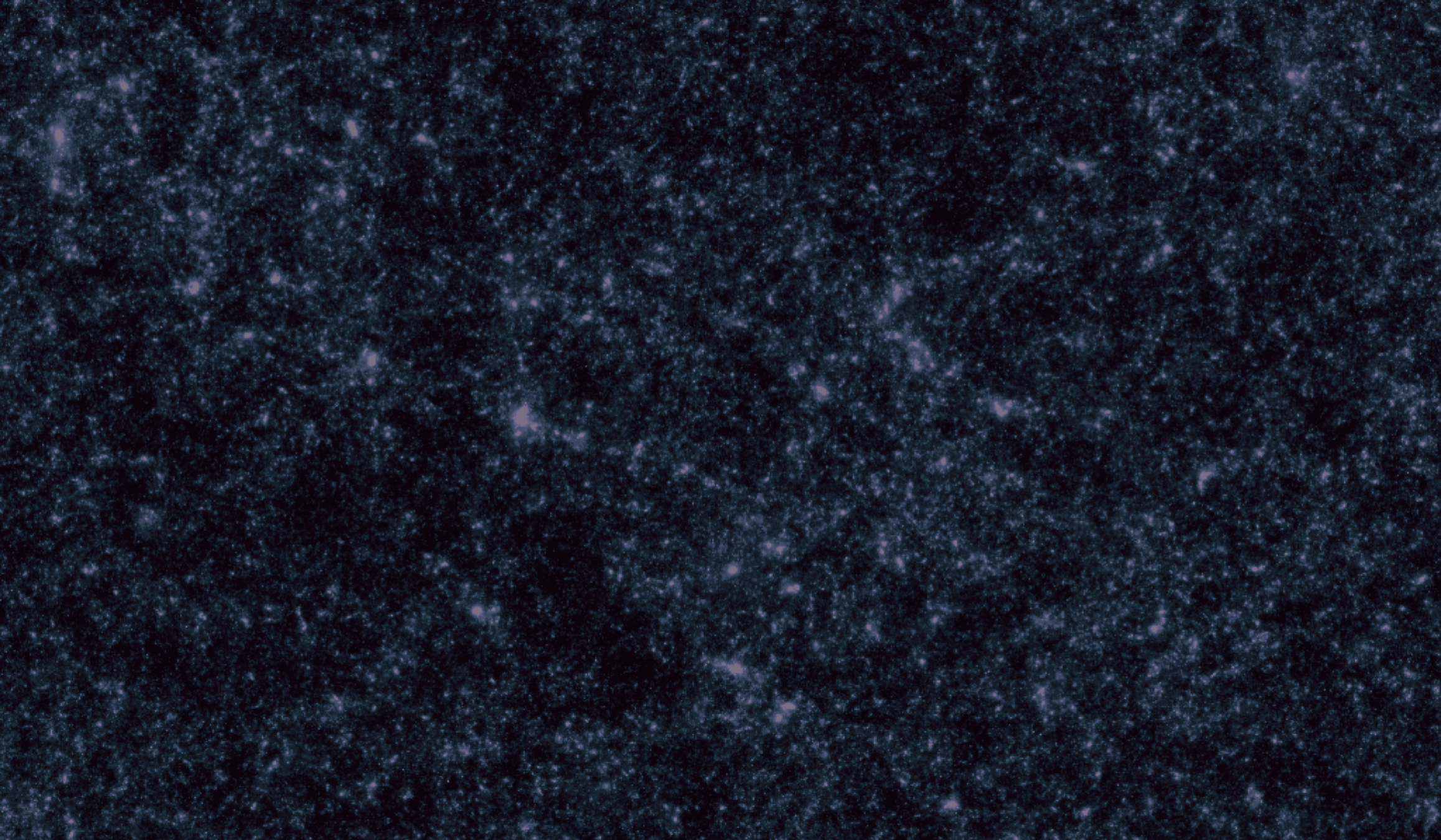
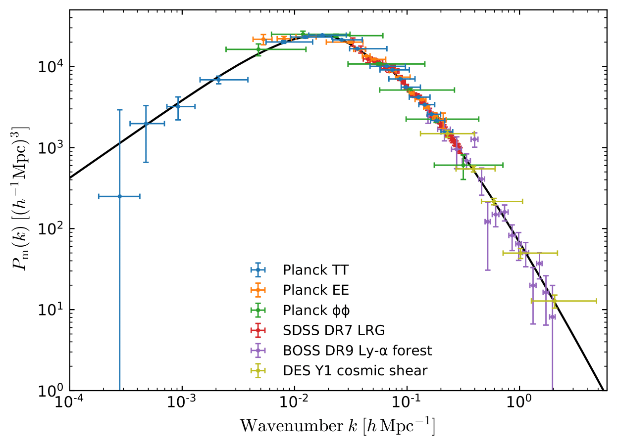
Cosmological context
ESA and the Planck Collaboration, 2018
\underbrace{p(\theta|x)}_{\text{posterior}}
\underbrace{p(\theta)}_{\text{prior}}
\underbrace{p(x|\theta)}_{\text{likelihood}}
\propto
Cosmological context
\underbrace{p(\theta|x)}_{\text{posterior}}
\underbrace{p(\theta)}_{\text{prior}}
\underbrace{p(x|\theta)}_{\text{likelihood}}
\propto
Cosmological context
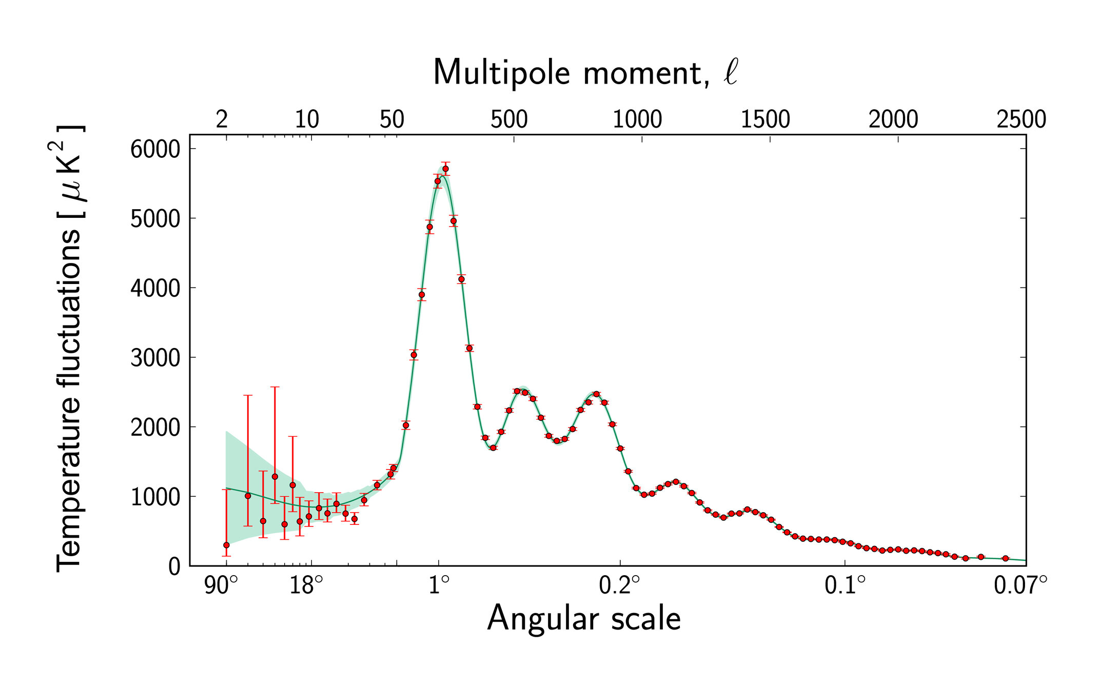
How to extract all the information embedded in our data?
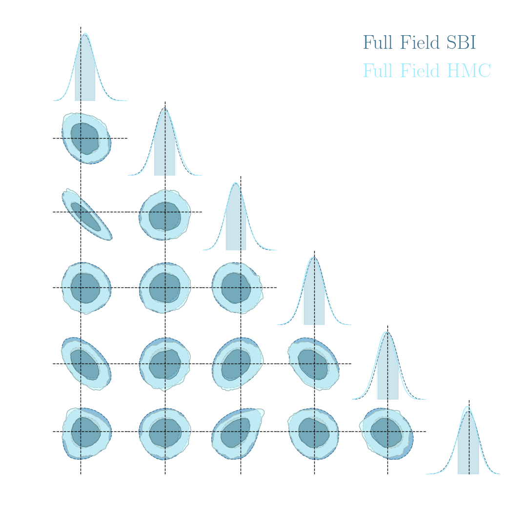
Full-Field Inference
working at the pixel level
Downsides:
-
Computationally expensive (HMC)
Our Goal: doing Neural Posterior Estimation (Implicit Inference) with a minimum number of simulations.
-
Require a large number of simulations
\underbrace{p(\theta|x)}_{\text{posterior}}
\underbrace{p(\theta)}_{\text{prior}}
\underbrace{p(x|\theta)}_{\text{likelihood}}
\propto
-
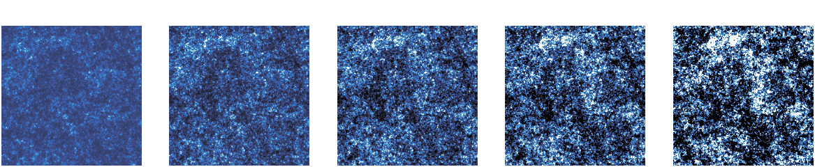
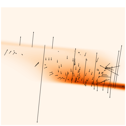
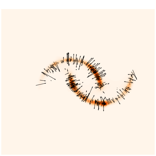
We developed a differentiable (JAX) log-normal mass maps simulator
Differentiable Mass Maps Simulator
-
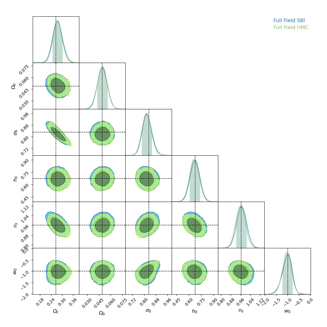
There is indeed more information to extract!
-
With infinite number of simulations, our Implicit Inference contours are as good as the Full-Field contours obtained through HMC

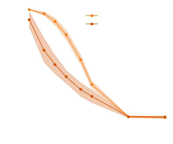
How can we reduce this number of simulations?
Gradient constraining power


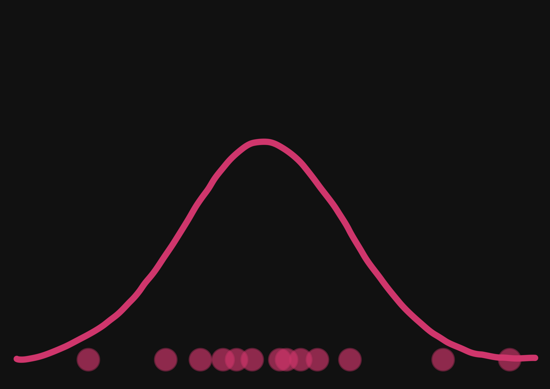
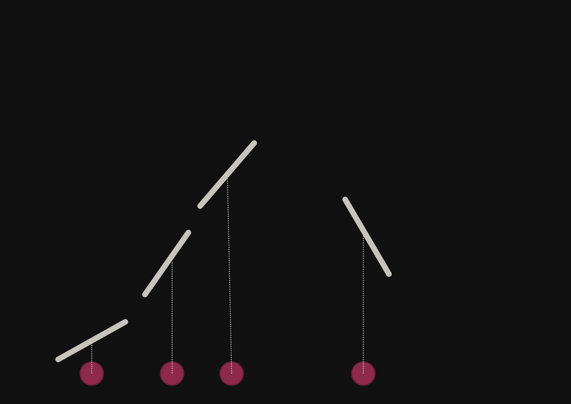
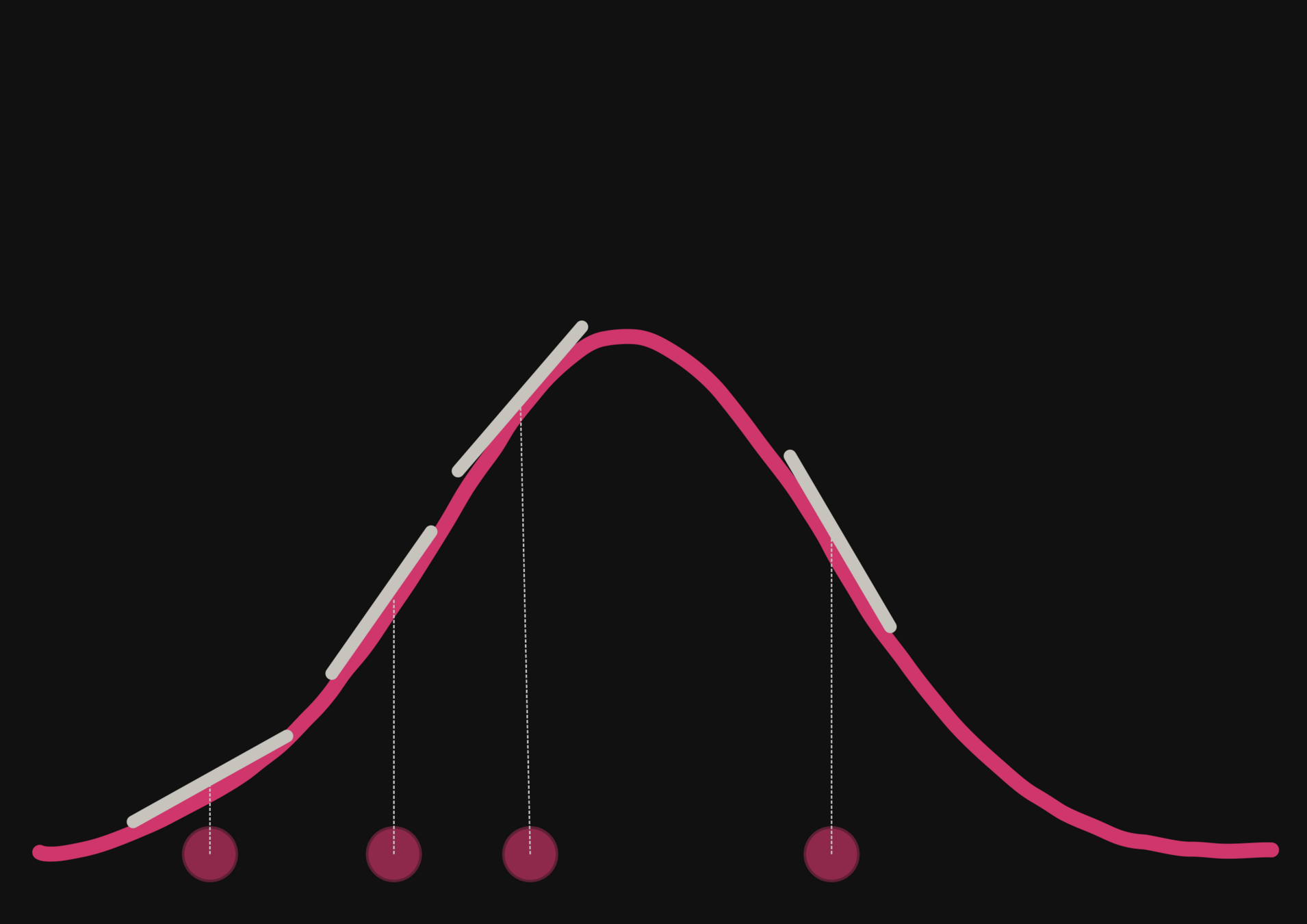
With a few simulations it's hard to approximate the posterior distribution.
→ we need more simulations
BUT if we have a few simulations
and the gradients
(also know as the score)
\nabla_{\theta} \log p(\theta|x)
Following this idea from Brehmer et al. 2019 we add the gradients of joint log probability of the simulator with respect to input parameters in the process
then it's possible to have an idea of the shape of the distribution.
Normalizing Flows (NFs) as Neural Density Estimators
Nfs are usually trained by minimizing the negative log likelihood loss:
- \mathbb{E}_{p(x)}\left[ \log\left(p_x^{\phi}(x)\right) \right]
- \mathbb{E}_{p(x)}\left[ \log\left(p_x^{\phi}(x)\right) \right]
Normalizing Flows (NFs) as Neural Density Estimators
- \mathbb{E}_{p(x)}\left[ \log\left(p_x^{\phi}(x)\right) \right]
But to train the NF, we want to use both simulations and gradients
Nfs are usually trained by minimizing the negative log likelihood loss:
- \mathbb{E}_{p(x)}\left[ \log\left(p_x^{\phi}(x)\right) \right]
Normalizing Flows (NFs) as Neural Density Estimators
- \mathbb{E}_{p(x)}\left[ \log\left(p_x^{\phi}(x)\right) \right]
+ \: \lambda \: \displaystyle \mathbb{E}\left[ \parallel \nabla_{x} \log p_x(x) - \underbrace{\nabla_x \log p_x^{\phi}(x)}\parallel_2^2 \right]
But to train the NF, we want to use both simulations and gradients
Nfs are usually trained by minimizing the negative log likelihood loss:
- \mathbb{E}_{p(x)}\left[ \log\left(p_x^{\phi}(x)\right) \right]
Normalizing Flows (NFs) as Neural Density Estimators
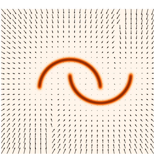
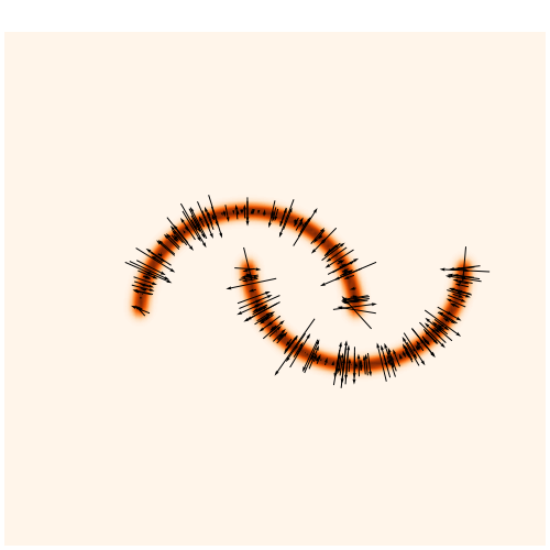
Problem: the gradient of current NFs lack expressivity
- \mathbb{E}_{p(x)}\left[ \log\left(p_x^{\phi}(x)\right) \right]
+ \: \lambda \: \displaystyle \mathbb{E}\left[ \parallel \nabla_{x} \log p_x(x) - \underbrace{\nabla_x \log p_x^{\phi}(x)}\parallel_2^2 \right]
But to train the NF, we want to use both simulations and gradients
Nfs are usually trained by minimizing the negative log likelihood loss:
- \mathbb{E}_{p(x)}\left[ \log\left(p_x^{\phi}(x)\right) \right]
Normalizing Flows (NFs) as Neural Density Estimators
Problem: the gradient of current NFs lack expressivity
Results from our previous paper
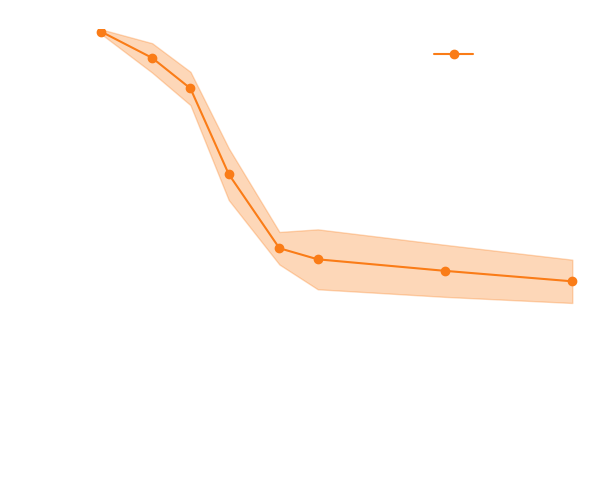
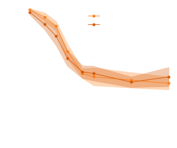
Wide proposal distribution
Narrow proposal distribution

→ The score helps to constrain the distribution shape
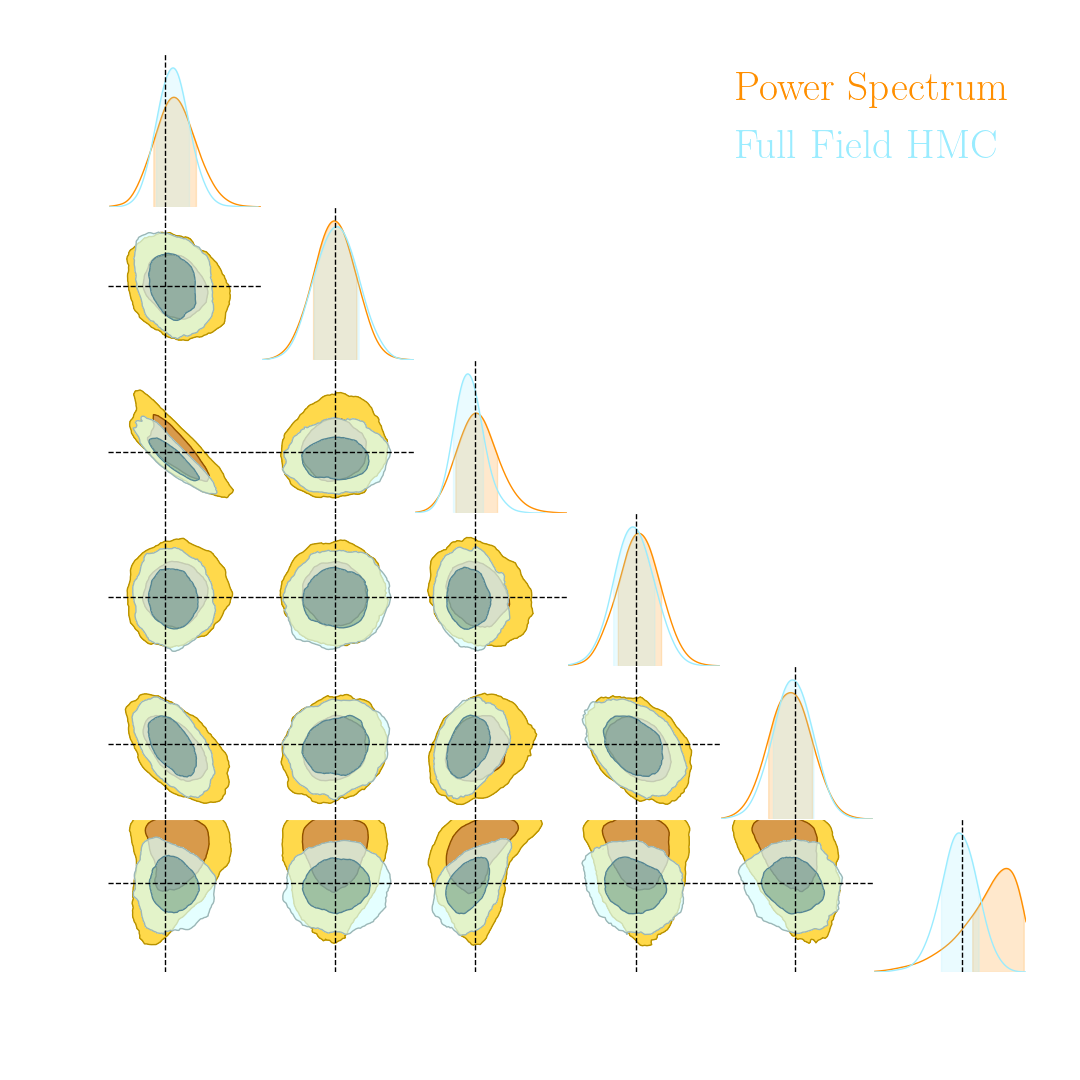
Cosmological application
Since the score helps to constrain the shape, we start from the power spectrum posterior
Cosmological application
Since the score helps to constrain the shape, we start from the power spectrum posterior
\frac{p(\theta) \: \tilde{p}(x)}{\tilde{p}(\theta) \: p(x)}
p(\theta | x) = \tilde{p}(\theta | x)
Cosmological application
Since the score helps to constrain the shape, we start from the power spectrum posterior
\frac{p(\theta) \: \tilde{p}(x)}{\tilde{p}(\theta) \: p(x)}
p(\theta | x) = \tilde{p}(\theta | x)
- \mathbb{E}_{p(x)}\left[ \log\left(p_x^{\phi}(x)\right) \right]
+ \: \lambda \: \displaystyle \mathbb{E}\left[ \parallel \nabla_{x} \log p_x(x) - \underbrace{\nabla_x \log p_x^{\phi}(x)}\parallel_2^2 \right]
We adapt the previous loss:
Cosmological application
Since the score helps to constrain the shape, we start from the power spectrum posterior
\frac{p(\theta) \: \tilde{p}(x)}{\tilde{p}(\theta) \: p(x)}
p(\theta | x) = \tilde{p}(\theta | x)
We adapt the previous loss:
- \mathbb{E}_{p(x)}\left[ \log\left(p_x^{\phi}(x)\right) \right]
+ \: \lambda \: \displaystyle \mathbb{E}\left[ \parallel \nabla_{x} \log p_x(x) - \underbrace{\nabla_x \log p_x^{\phi}(x)}\parallel_2^2 \right]
Preliminary
Summary
\underbrace{p(\theta|x)}_{\text{posterior}}
\underbrace{p(\theta)}_{\text{prior}}
\underbrace{p(x|\theta)}_{\text{likelihood}}
\propto
Summary
\underbrace{p(\theta|x)}_{\text{posterior}}
\underbrace{p(\theta)}_{\text{prior}}
\underbrace{p(x|\theta)}_{\text{likelihood}}
\propto
Goal: approximate the posterior
Summary
Problem: we don't have an analytic marginalized likelihood
Goal: approximate the posterior
\underbrace{p(\theta|x)}_{\text{posterior}}
\underbrace{p(x|\theta)}_{\text{likelihood}}
\underbrace{p(\theta)}_{\text{prior}}
\propto
Summary
Current methods: insufficient summary statistics + gaussian assumptions
Goal: approximate the posterior
\underbrace{p(\theta|x)}_{\text{posterior}}
\underbrace{p(\theta)}_{\text{prior}}
\underbrace{p(x|\theta)}_{\text{likelihood}}
\propto
Problem: we don't have an analytic marginalized likelihood
Summary
→ need new methods to extract all informations
\underbrace{p(\theta|x)}_{\text{posterior}}
\underbrace{p(\theta)}_{\text{prior}}
\underbrace{p(x|\theta)}_{\text{likelihood}}
\propto
Current methods: insufficient summary statistics + gaussian assumptions
Goal: approximate the posterior
Problem: we don't have an analytic marginalized likelihood
Summary
\underbrace{p(\theta|x)}_{\text{posterior}}
\underbrace{p(\theta)}_{\text{prior}}
\underbrace{p(x|\theta)}_{\text{likelihood}}
\propto
→ Full-Field Inference
→ need new methods to extract all informations
Current methods: insufficient summary statistics + gaussian assumptions
Goal: approximate the posterior
Problem: we don't have an analytic marginalized likelihood
Summary
→ computationally expensive + large number of simulations
\underbrace{p(\theta|x)}_{\text{posterior}}
\underbrace{p(\theta)}_{\text{prior}}
\underbrace{p(x|\theta)}_{\text{likelihood}}
\propto
→ Full-Field Inference
→ need new methods to extract all informations
Current methods: insufficient summary statistics + gaussian assumptions
Goal: approximate the posterior
Problem: we don't have an analytic marginalized likelihood
Summary
directly approximate the posterior (NPE): no need for MCMCs
\underbrace{p(\theta|x)}_{\text{posterior}}
\underbrace{p(\theta)}_{\text{prior}}
\underbrace{p(x|\theta)}_{\text{likelihood}}
\propto
→
→ computationally expensive + large number of simulations
→ Full-Field Inference
→ need new methods to extract all informations
Current methods: insufficient summary statistics + gaussian assumptions
Goal: approximate the posterior
Problem: we don't have an analytic marginalized likelihood
directly approximate the posterior (NPE): no need for MCMCs
Summary
\underbrace{p(\theta|x)}_{\text{posterior}}
\underbrace{p(\theta)}_{\text{prior}}
\underbrace{p(x|\theta)}_{\text{likelihood}}
\propto
directly approximate the posterior (NPE): no need for MCMCs
→
→ computationally expensive + large number of simulations
→ Full-Field Inference
→ need new methods to extract all informations
Current methods: insufficient summary statistics + gaussian assumptions
Goal: approximate the posterior
Problem: we don't have an analytic marginalized likelihood
directly approximate the posterior (NPE): no need for MCMCs
SBI with gradients
→
Summary
\underbrace{p(\theta|x)}_{\text{posterior}}
\underbrace{p(\theta)}_{\text{prior}}
\underbrace{p(x|\theta)}_{\text{likelihood}}
\propto
directly approximate the posterior (NPE): no need for MCMCs
→
→ computationally expensive + large number of simulations
→ Full-Field Inference
→ need new methods to extract all information
Current methods: insufficient summary statistics + gaussian assumptions
Goal: approximate the posterior
Problem: we don't have an analytic marginalized likelihood
directly approximate the posterior (NPE): no need for MCMCs
SBI with gradients
→
⚠️ requirements: differentiable simulator + smooth NDE
Summary
\underbrace{p(\theta|x)}_{\text{posterior}}
\underbrace{p(\theta)}_{\text{prior}}
\underbrace{p(x|\theta)}_{\text{likelihood}}
\propto
directly approximate the posterior (NPE): no need for MCMCs
→
→ computationally expensive + large number of simulations
→ Full-Field Inference
→ need new methods to extract all information
Current methods: insufficient summary statistics + gaussian assumptions
Goal: approximate the posterior
Problem: we don't have an analytic marginalized likelihood
directly approximate the posterior (NPE): no need for MCMCs
Thank You!
⚠️ requirements: differentiable simulator + smooth NDE
SBI with gradients
→
talk cca 2023
By Justine Zgh


