Field-Level
Inference
Justine Zeghal
justine.zeghal@umontreal.ca
Learning the Universe meeting
October 2025
Université de Montréal
\underbrace{p(\theta|x=x_0)}_{\text{posterior}}
\underbrace{p(\theta)}_{\text{prior}}
\underbrace{p(x = x_0|\theta)}_{\text{likelihood}}
\propto
Bayes theorem:
We can build a simulator to map the cosmological parameters to the data.
Prediction
Inference
Full-field inference: extracting all cosmological information
x
\theta
Simulator
\underbrace{p(x = x_0|\theta)}_{\text{likelihood}}
Depending on the simulator’s nature we can either perform
- Explicit inference
- Implicit inference
Full-field inference: extracting all cosmological information
\theta
Simulator
z
x
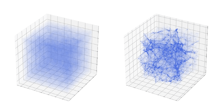
Initial conditions of the Universe
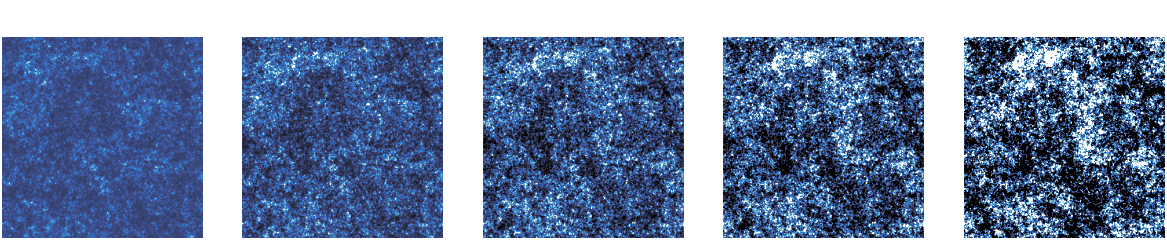
Large Scale Structure
p(\theta, z \: | \: x) \propto
p(z\:|\:\theta) p(\theta)
Needs an explicit simulator to sample the joint posterior through MCMC:
p(x| \theta, z)
We need to sample in
high-dimension
→ gradient-based sampling schemes
z
f
\sigma^2
\mathcal{N}
-
Explicit inference
x
Explicit joint likelihood
p(x| \theta, z)
(\theta_i, x_i)_{i=1...N}
This approach typically involve 2 steps:
2) Implicit inference on these summary statistics to approximate the posterior.
1) compression of the high dimensional data into summary statistics. Without loosing cosmological information!
Summary statistics
t = f_{\varphi}(x)
p_{\Phi}(\theta | f_{\varphi}(x))
Full-field inference: extracting all cosmological information
\theta
Simulator
-
Implicit inference
It does not matter if the simulator is explicit or implicit because all we need are simulations
x
Outline
Which full-field inference methods require the fewest simulations?
How to build sufficient statistics?
Can we perform implicit inference with fewer simulations?
How to generate more realistic simulations?
Outline
Which full-field inference methods require the fewest simulations?
How to build sufficient statistics?
Can we perform implicit inference with fewer simulations?
How to generate more realistic simulations?
Optimal Neural Summarisation for Full-Field Weak Lensing Cosmological Implicit Inference
Denise Lanzieri*, Justine Zeghal*, T. Lucas Makinen, François Lanusse, Alexandre Boucaud and Jean-Luc Starck

t = f_{\varphi}(x)
\theta
p(\theta \: | \: x) = p(\theta \: | \: t) \: \text{ with } \: t=f(x)
It is only a matter of the loss function used to train the compressor.
How to extract all the information?
Sufficient Statistic
A statistic t is said to be sufficient for the parameters if and only if
x
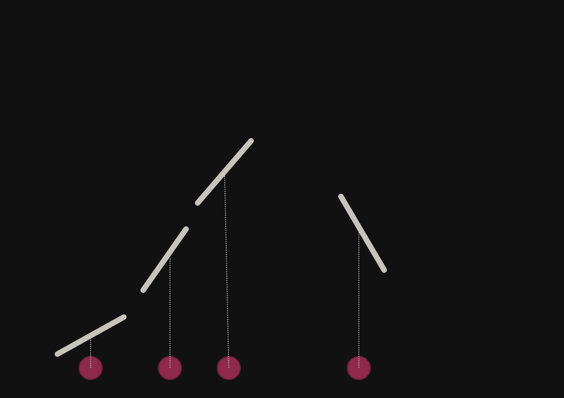
Two main compression schemes
\hat{\theta} = f_\varphi(x)
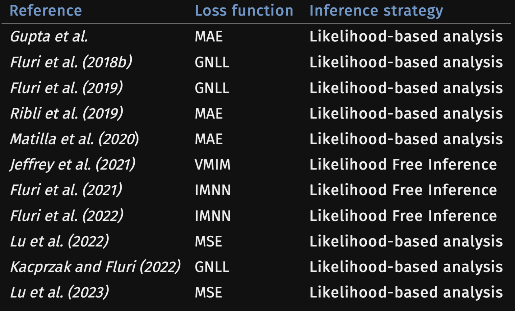
Regression Losses
Two main compression schemes
\hat{\theta} = f_\varphi(x)
Regression Losses
Which learns a moment of the posterior distribution.
Two main compression schemes
Mean Squared Error (MSE) loss:
\mathcal{L}_{\text{MSE}} = \mathbb{E}_{p(x,\theta)} \left[\parallel \theta - f_\varphi(x) \parallel ^2 \right]
Which learns a moment of the posterior distribution.
\hat{\theta} = f_\varphi(x)
Regression Losses
Two main compression schemes
\mathcal{L}_{\text{MSE}} = \mathbb{E}_{p(x,\theta)} \left[\parallel \theta - f_\varphi(x) \parallel ^2 \right]
→ Approximate the mean of the posterior.
\hat{\theta} = f_\varphi(x)
Which learns a moment of the posterior distribution.
Two main compression schemes
Mean Squared Error (MSE) loss:
Regression Losses
\mathcal{L}_{\text{MSE}} = \mathbb{E}_{p(x,\theta)} \left[\parallel \theta - f_\varphi(x) \parallel ^2 \right]
→ Approximate the mean of the posterior.
\hat{\theta} = f_\varphi(x)
Mean Absolute Error (MAE) loss:
\mathcal{L}_{\text{MAE}} = \mathbb{E}_{p(x,\theta)} \left[| \theta - f_\varphi(x) |\right]
Which learns a moment of the posterior distribution.
Two main compression schemes
Mean Squared Error (MSE) loss:
Regression Losses
→ Approximate the median of the posterior.
Two main compression schemes
\mathcal{L}_{\text{MSE}} = \mathbb{E}_{p(x,\theta)} \left[\parallel \theta - f_\varphi(x) \parallel ^2 \right]
→ Approximate the mean of the posterior.
\hat{\theta} = f_\varphi(x)
Mean Absolute Error (MAE) loss:
\mathcal{L}_{\text{MAE}} = \mathbb{E}_{p(x,\theta)} \left[| \theta - f_\varphi(x) |\right]
Which learns a moment of the posterior distribution.
Mean Squared Error (MSE) loss:
Regression Losses
Regression Losses
Two main compression schemes
\mu_1 = \mu_2
Two main compression schemes
Regression Losses
\mu_1 = \mu_2
Two main compression schemes
Regression Losses
\mu_1 = \mu_2
Two main compression schemes
Regression Losses
\mu_1 = \mu_2
\neq
The mean is not guaranteed to be a sufficient statistic.
Two main compression schemes
Regression Losses
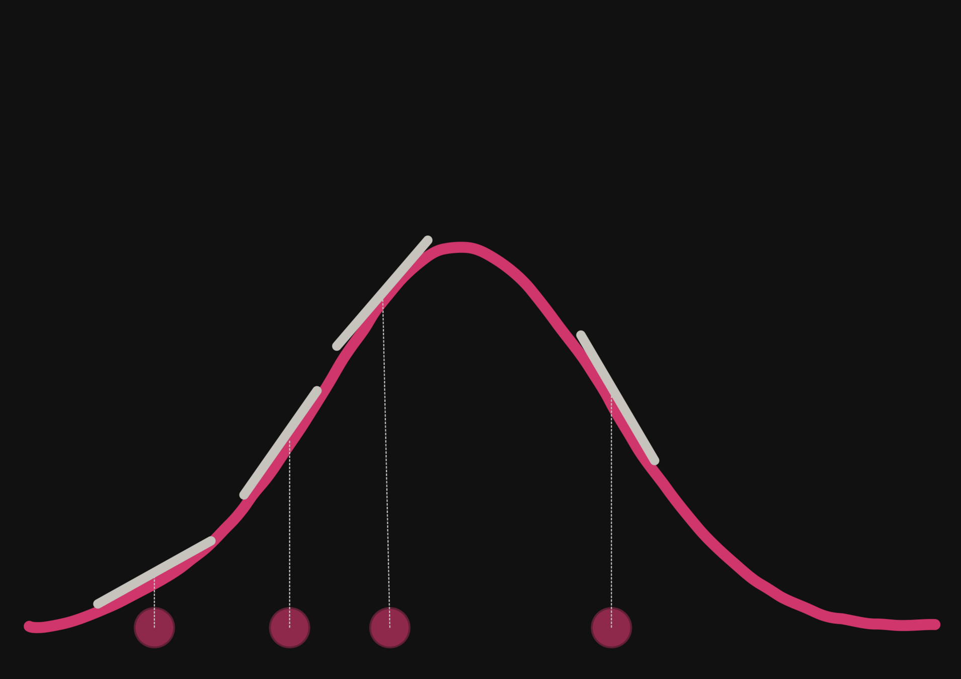
Mutual information maximization
Two main compression schemes
p(\theta \: | \: x) = p(\theta \: | \: t(x)) \: \Leftrightarrow I(\theta, x) = I (\theta, t(x))
Mutual information maximization
By definition:
Two main compression schemes
I(\theta,x)
H(\theta)
H(x)
H(\theta|x)
H(x|\theta)
I(\theta,x) = H(x) - H(x|\theta)
p(\theta \: | \: x) = p(\theta \: | \: t(x)) \: \Leftrightarrow I(\theta, x) = I (\theta, t(x))
Mutual information maximization
By definition:
Two main compression schemes
p(\theta \: | \: x) = p(\theta \: | \: t(x)) \: \Leftrightarrow I(\theta, x) = I (\theta, t(x))
Mutual information maximization
By definition:
Two main compression schemes
I(\theta,x)
H(\theta)
H(x)
H(\theta|x)
H(x|\theta)
I(\theta,x) = H(x) - H(x|\theta)
p(\theta \: | \: x) = p(\theta \: | \: t(x)) \: \Leftrightarrow I(\theta, x) = I (\theta, t(x))
Mutual information maximization
By definition:
Two main compression schemes
I(\theta,x)
H(\theta)
H(x)
H(\theta|x)
H(x|\theta)
I(\theta,x) = H(x) - H(x|\theta)
p(\theta \: | \: x) = p(\theta \: | \: t(x)) \: \Leftrightarrow I(\theta, x) = I (\theta, t(x))
Mutual information maximization
By definition:
Two main compression schemes
I(\theta,x)
H(\theta)
H(x)
H(\theta|x)
H(x|\theta)
I(\theta,x) = H(x) - H(x|\theta)
p(\theta \: | \: x) = p(\theta \: | \: t(x)) \: \Leftrightarrow I(\theta, x) = I (\theta, t(x))
Mutual information maximization
By definition:
Two main compression schemes
I(\theta,x)
H(\theta)
H(x)
H(\theta|x)
H(x|\theta)
I(\theta,x) = H(x) - H(x|\theta)
→ build sufficient statistics according to the definition.
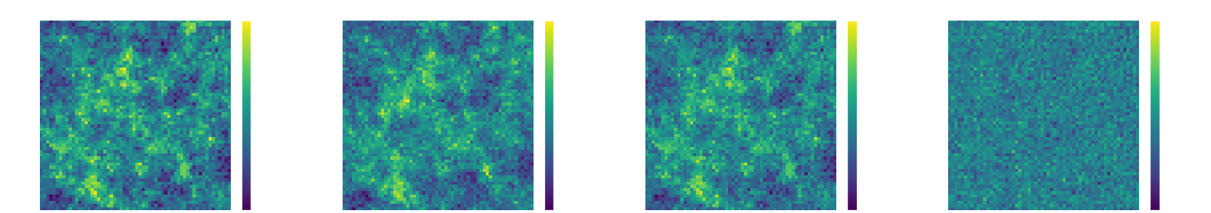
We developed a fast and differentiable (JAX) log-normal mass maps simulator.
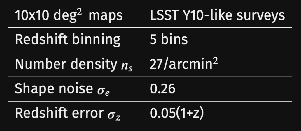

For our benchmark: a Differentiable Mass Maps Simulator
1. We compress using one of the losses.
Benchmark procedure:
2. We compare their extraction power by comparing their posteriors.
For this, we use implicit inference, which is fixed for all the compression strategies.
p(\theta \: | \: x) = p(\theta \: | \: t) \: \text{ with } \: t=f(x)
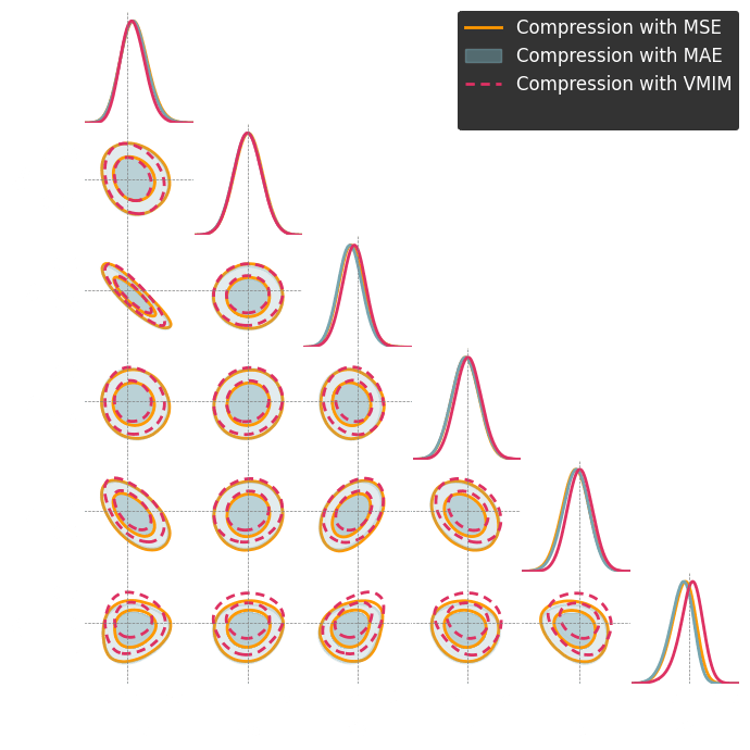
Numerical results
Outline
Which full-field inference methods require the fewest simulations?
How to build sufficient statistics?
Can we perform implicit inference with fewer simulations?
How to generate more realistic simulations?
Outline
Which full-field inference methods require the fewest simulations?
How to build sufficient statistics?
Can we perform implicit inference with fewer simulations?
How to generate more realistic simulations?
Neural Posterior Estimation with Differentiable Simulators
ICML 2022 Workshop on Machine Learning for Astrophysics
Justine Zeghal, François Lanusse, Alexandre Boucaud,
Benjamin Remy and Eric Aubourg
Neural Posterior Estimation
There exist several ways to do implicit inference
(\theta_i, x_i)_{i=1...N} \sim p(x, \theta)
- Learning the likelihood
- Learning the likelihood ratio
- Learning the posterior
Neural Posterior Estimation
→ Normalizing Flows
\begin{array}{ll}
Loss = - \mathbb{E}_{p(x, \theta)}\left[ \log\left(p^{\phi}(\theta\mid x)\right) \right]\\
\end{array}
From simulations only!
A lot of simulations..
There exist several ways to do implicit inference
(\theta_i, x_i)_{i=1...N} \sim p(x, \theta)
- Learning the likelihood
- Learning the likelihood ratio
- Learning the posterior
Neural Posterior Estimation with Gradients


→ Normalizing Flows
\begin{array}{ll}
Loss = - \mathbb{E}_{p(x, \theta)}\left[ \log\left(p^{\phi}(\theta\mid x)\right) \right]\\
\end{array}
From simulations only!
A lot of simulations..
There exist several ways to do implicit inference
(\theta_i, x_i)_{i=1...N} \sim p(x, \theta)
How gradients can help reduce the number of simulations?
(\theta_i, x_i, \nabla_\theta \log p(\theta \mid x_i))_{i=1...N}
- Learning the likelihood
- Learning the likelihood ratio
- Learning the posterior
Normalizing Flows training with gradients
Normalizing flows are trained by minimizing the negative log likelihood:
- \mathbb{E}_{p(x, \theta)}\left[ \log\left(p^{\phi}(\theta | x)\right) \right]
Normalizing Flows training with gradients
But to train the NF, we want to use both simulations and the gradients from the simulator
- \mathbb{E}_{p(x, \theta)}\left[ \log\left(p^{\phi}(\theta | x)\right) \right]
Normalizing flows are trained by minimizing the negative log likelihood:
- \mathbb{E}_{p(x, \theta)}\left[ \log\left(p^{\phi}(\theta | x)\right) \right]
Normalizing Flows training with gradients
- \mathbb{E}_{p(x, \theta)}\left[ \log\left(p^{\phi}(\theta | x)\right) \right]
But to train the NF, we want to use both simulations and the gradients from the simulator
Normalizing flows are trained by minimizing the negative log likelihood:
- \mathbb{E}_{p(x, \theta)}\left[ \log\left(p^{\phi}(\theta | x)\right) \right]
Normalizing Flows training with gradients
+ \: \lambda \: \displaystyle \mathbb{E}\left[ \parallel \nabla_{\theta} \log p(\theta, z |x) - \nabla_{\theta} \log p^{\phi}(\theta |x)\parallel_2^2 \right]


→ On a toy Lotka Volterra model, the gradients helps to constrain the distribution shape.
- \mathbb{E}_{p(x, \theta)}\left[ \log\left(p^{\phi}(\theta | x)\right) \right]
But to train the NF, we want to use both simulations and the gradients from the simulator
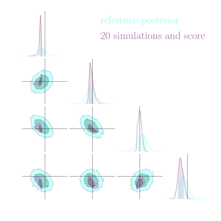
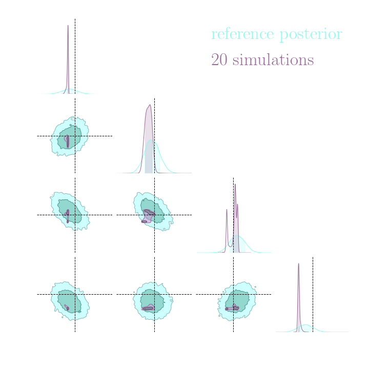
Without gradients
With gradients
Posteriors on a toy model
Outline
Which full-field inference methods require the fewest simulations?
How to build sufficient statistics?
Can we perform implicit inference with fewer simulations?
How to generate more realistic simulations?
Outline
Which full-field inference methods require the fewest simulations?
How to build sufficient statistics?
Can we perform implicit inference with fewer simulations?
How to generate more realistic simulations?
Simulation-Based Inference Benchmark for Weak Lensing Cosmology
Justine Zeghal, Denise Lanzieri, François Lanusse, Alexandre Boucaud, Gilles Louppe, Eric Aubourg, Adrian E. Bayer
and The LSST Dark Energy Science Collaboration (LSST DESC)
We developed a fast and differentiable (JAX) log-normal mass maps simulator.
For our benchmark: a Differentiable Mass Maps Simulator
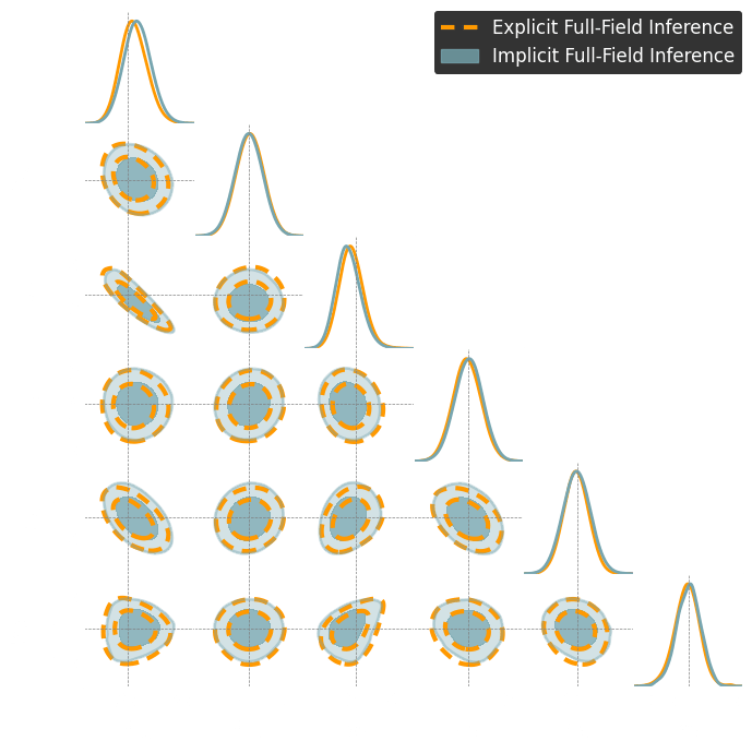
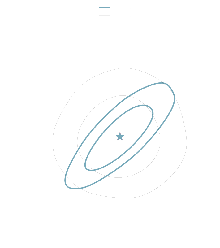
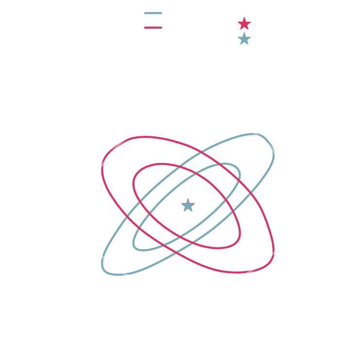
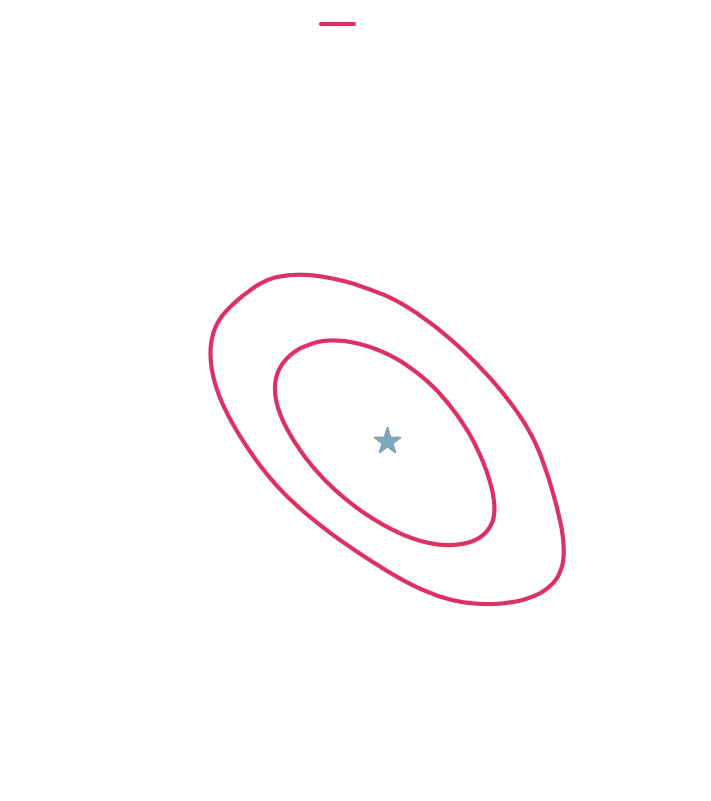
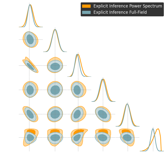
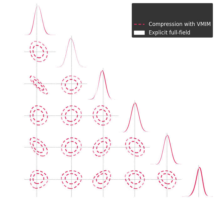
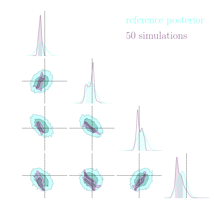
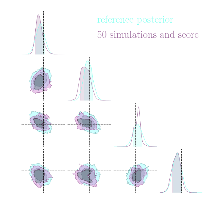
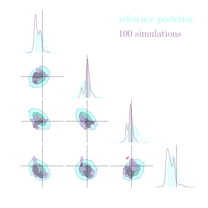
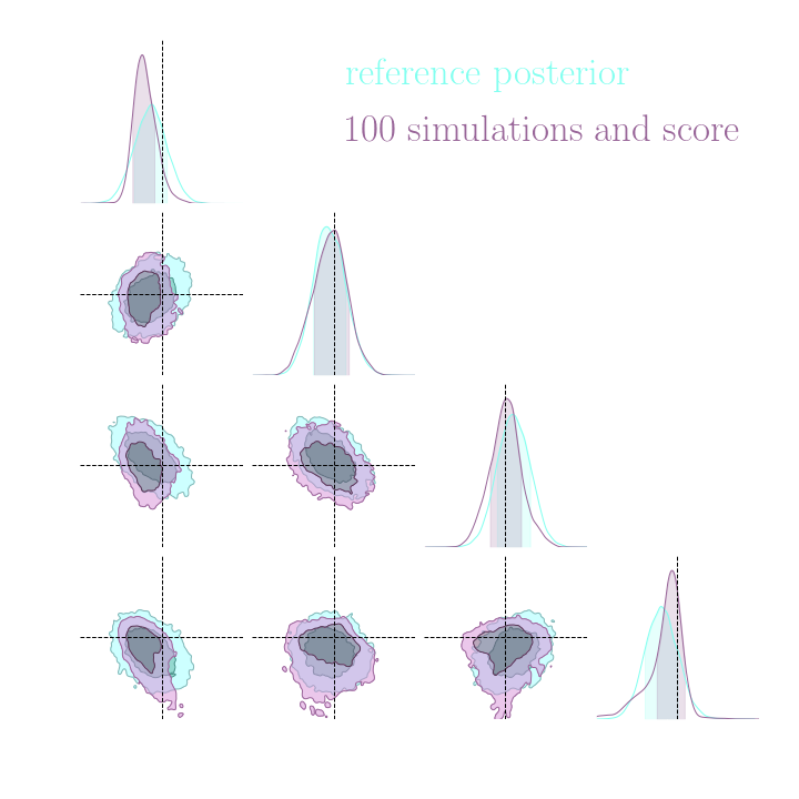
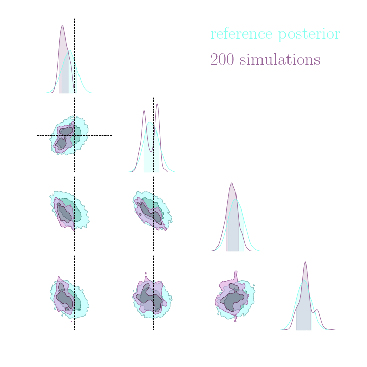
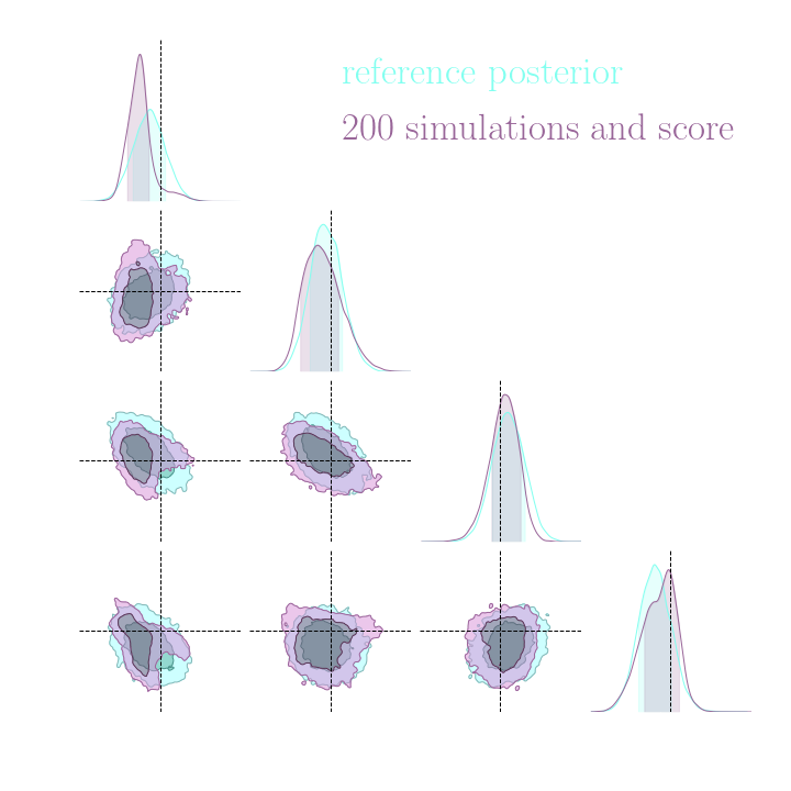
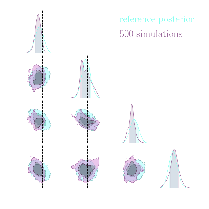
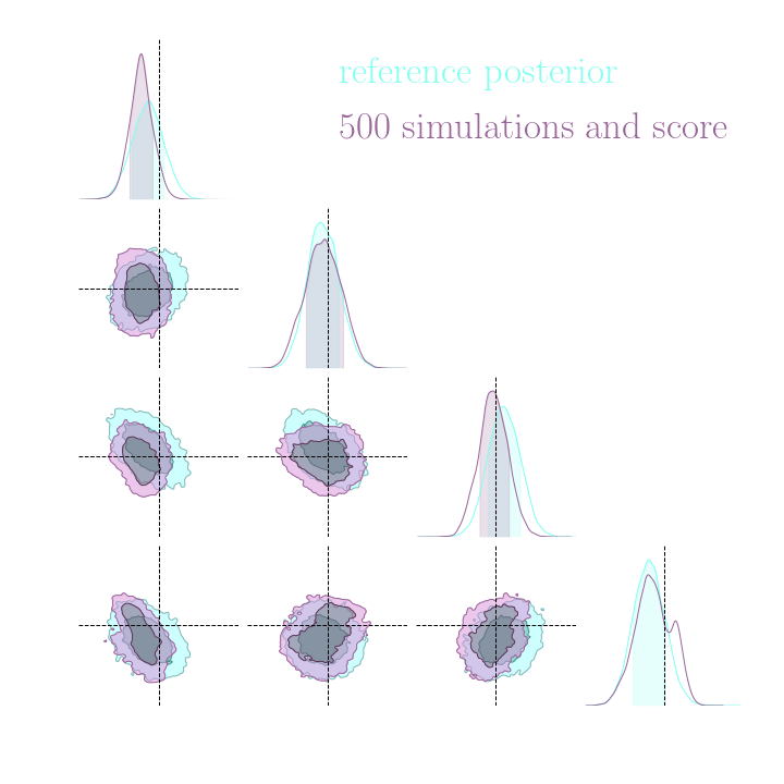
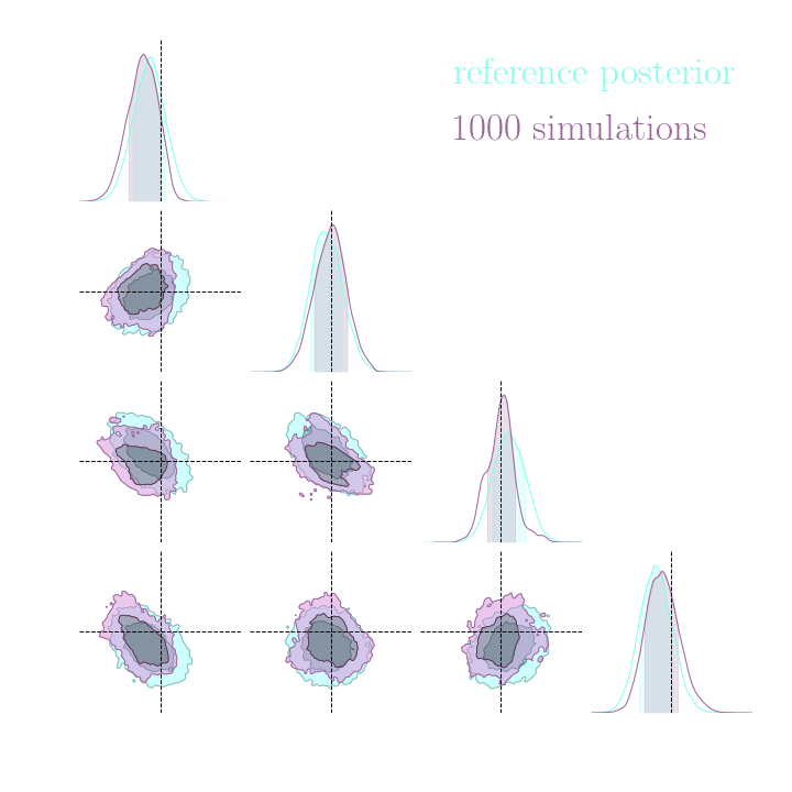
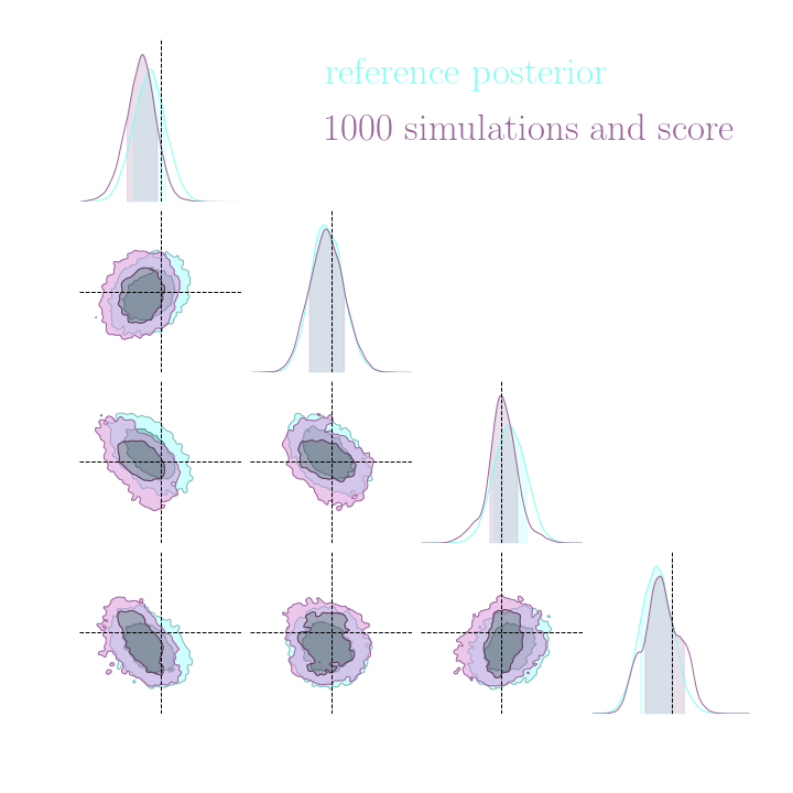
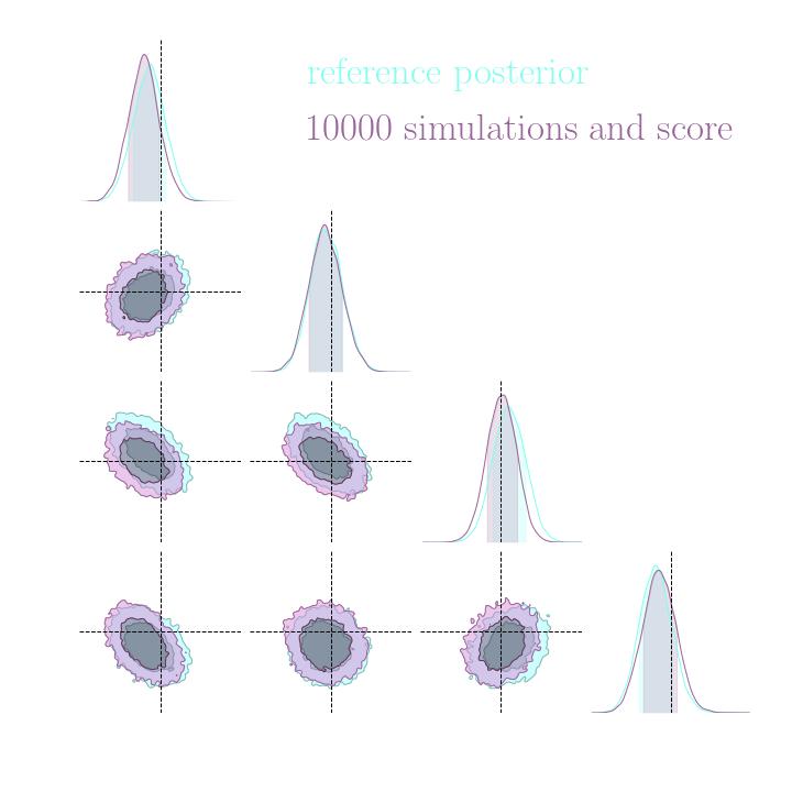
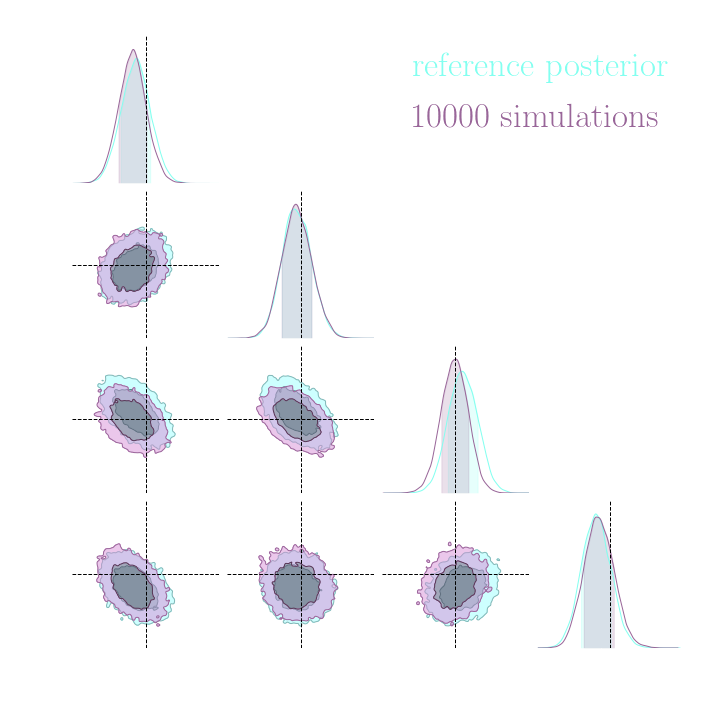
Benchmark Results
Both explicit and implicit inference yield the same posterior.
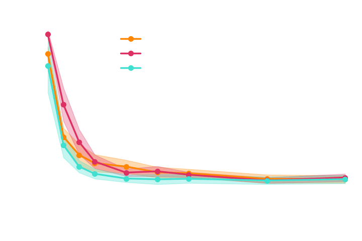
The gradients are too noisy to help reduce the number of simulations in implicit inference.
Implicit inference needs 10^3 simulations.
\displaystyle \mathbb{E}\left[ \parallel \nabla_{\theta} \log p(\theta, z |x) - \nabla_{\theta} \log p^{\phi}(\theta |x)\parallel_2^2 \right]
Benchmark Results
Both explicit and implicit inference yield the same posterior.
Explicit inference needs 10^6 simulations.
The gradients are too noisy to help reduce the number of simulations in implicit inference.
Implicit inference needs 10^3 simulations.
- \mathbb{E}_{p(x, \theta)}\left[ \log\left(p^{\phi}(x | \theta)\right) \right]
+ \: \lambda \: \displaystyle \mathbb{E}\left[ \parallel \nabla_{\theta} \log p(x, z |\theta) -{\nabla_{\theta} \log p^{\phi}(x|\theta )}\parallel_2^2 \right]
Training the NF with simulations and gradients:
Loss =
-
Do gradients help implicit inference methods?

- \mathbb{E}_{p(x, \theta)}\left[ \log\left(p^{\phi}(x | \theta)\right) \right]
Training the NF with simulations and gradients:
Loss =
-
Do gradients help implicit inference methods?
(\theta_i, x_i)_{i=1...N}
\nabla_{\theta} \log \hat{p}(x |\theta)

+ \: \lambda \: \displaystyle \mathbb{E}\left[ \parallel \nabla_{\theta} \log p(x, z |\theta) -{\nabla_{\theta} \log p^{\phi}(x|\theta )}\parallel_2^2 \right]
Outline
Which full-field inference methods require the fewest simulations?
How to build sufficient statistics?
Can we perform implicit inference with fewer simulations?
How to generate more realistic simulations?
Outline
Which full-field inference methods require the fewest simulations?
How to build sufficient statistics?
Can we perform implicit inference with fewer simulations?
How to generate more realistic simulations?
Bridging Simulators with Conditional Optimal Transport
Justine Zeghal, Benjamin Remy, Yashar Hezaveh, François Lanusse,
Laurence Perreault-Levasseur
ICML co-located 2024 Workshop on Machine Learning for Astrophysics
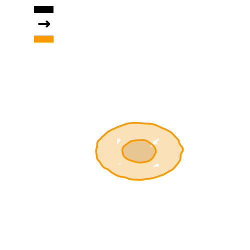
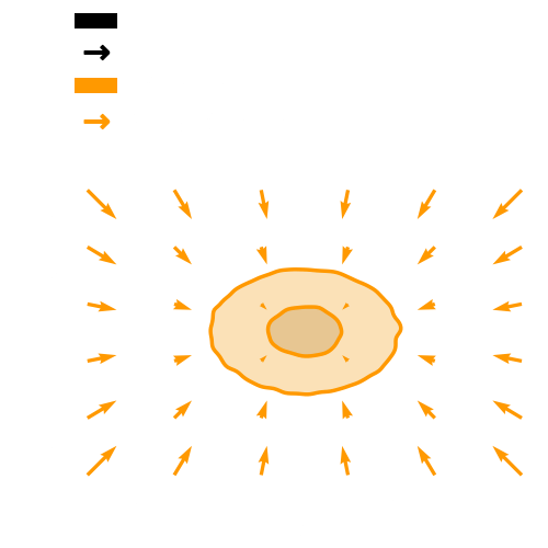
A way to emulate is to learn the correction of a cheap simulation:
= \phi_1( \:\:\:\:\:\:\:\:\:)
→ OT Flow Matching enables to learn an Optimal Transport mapping between two random distributions.
Easier than learning the entire simulation evolution.
We want:
- the transformation to minimally transform the simulation
- learning a conditional transformation
- work with unpaired dataset
Learning emulators to generate more simulations
With full-field inference, we are now only relying on simulations.
→ We need very realistic simulations.


Flow Matching
Flow Matching
Flow Matching
Flow Matching


Optimal Transport Flow Matching

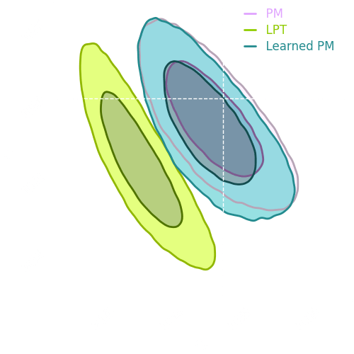
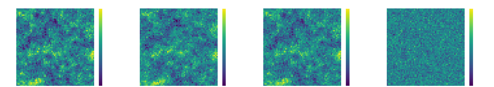
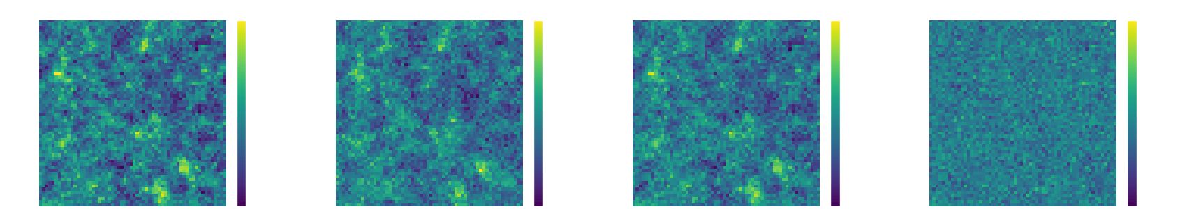
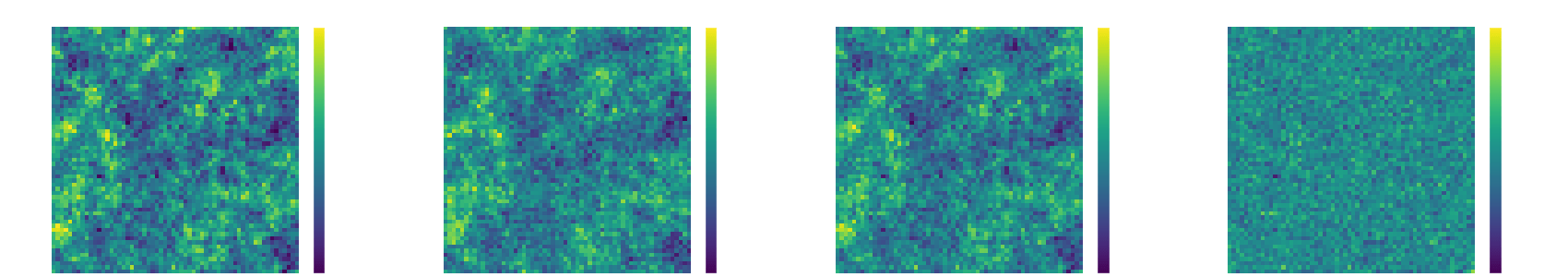
Results
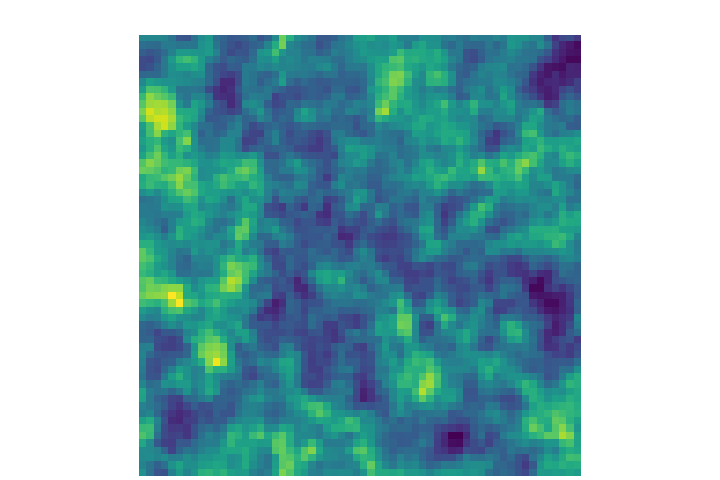
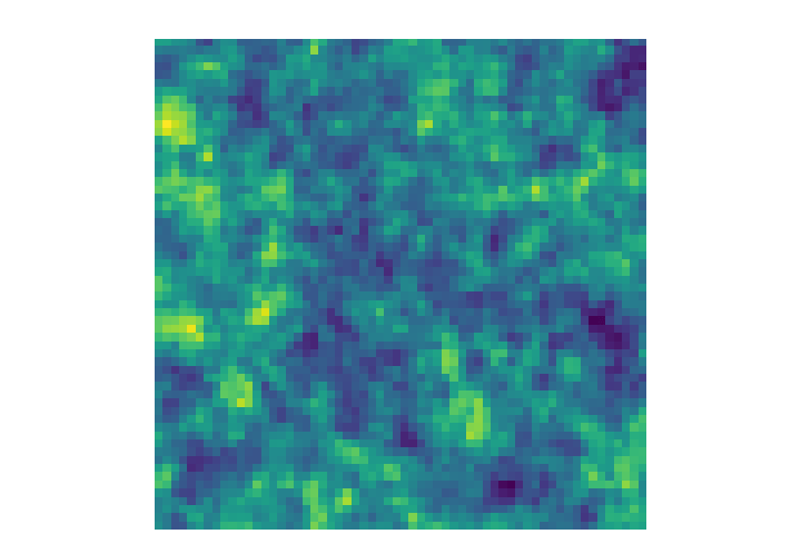
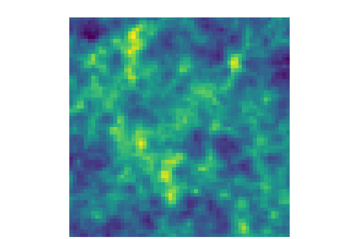
\theta
OT
\phi_1
\theta
LPT
PM
Experiment
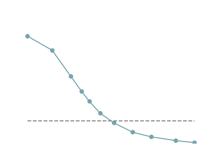
→ Good emulation
at the pixel-level
→ We can perform both implicit and explicit inference
Conclusion
Which full-field inference methods require the fewest simulations?
Can we perform implicit inference with fewer simulations?
How to build emulators?
Gradients can be beneficial, depending on your simulation model.
Explicit inference requires 100 times more simulations than implicit inference.
We can learn an optimal transport mapping.
How to build sufficient statistics?
Mutual Information Maximization
Thank you for your attention!
Summary statistics
t = f_{\varphi}(x)
p_{\Phi}(\theta | f_{\varphi}(x))
\theta
Simulator
x
Ltu meeting
By Justine Zgh


