week 05
Network Models
Social Network Analysis
Network Models
Empirical network features:
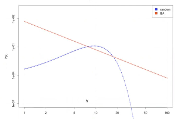
- Power-law (heavy-tailed) degree distribution
- Small average distance (graph diameter)
- Large clustering coefficient (transitivity)
Generative models:
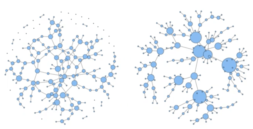
- Random graph model (Erdos & Renyi, 1959)
- Preferential attachment model (Barabasi & Albert, 1999)
- Small world model (Watts & Strogatz, 1998)
04-1
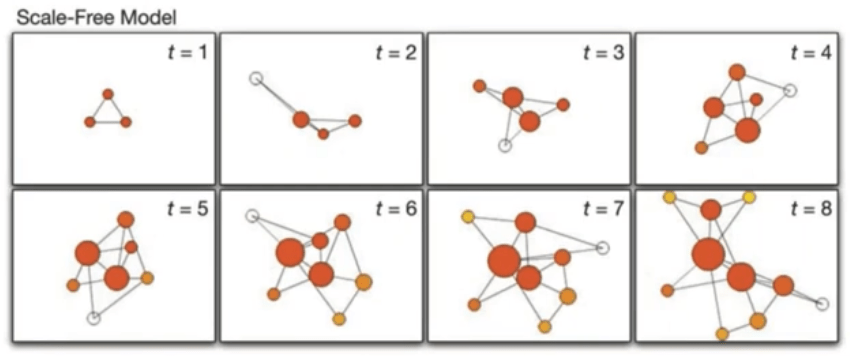
Prefferential Attachment
Preferential attachment model
Barabasi and Albert, 1999
Dynamic growth: start at \( t \) = 0 with по nodes and \( m_0 \geq n_0 \) edges
At each time step add a new node with \( m \) edges \( (m \leq n_0) \),
connecting to \( m \) nodes already in netwrok \( k_i(i) = m \)
The probability of linking to existing node i is proportional to
the node degree \( k_i \)
after \( t \) timesteps: \( t + n_0 \) nodes, \( mt + m_0 \) edges
1. Growth
2. Preferential attachment
П(k_i) = \frac{k_i}{\sum_ik_i}
Preferential attachment model
Preferential attachment model
Continues approximation: continues time, real variable node degree \( \langle k_j(t) \rangle \) - expected value over multiple realizations
node \( i \) is added at time \( t_i \) : \( k_i (t_i) = m \)
Solution:
\frac{dk_i(t)}{dt} = m П(k_i) = m \frac{k_i}{\sum_ik_i}=\frac{mk_i}{2mt}=\frac{k_i}{2t}
k_i(t + \delta t) = k_i(t) + m П(k_i)\delta t
\int_m^{k_i(t)} \frac{dk_i}{k_i} = \int_{t_i}^t \frac{dt}{2t}
k_i(t) = m ( \frac{t}{t_i})^{1/2}
Preferential attachment model
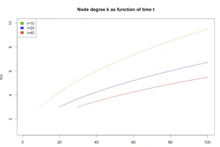
k_i(t) = m ( \frac{t}{t_i})^{1/2}
\frac{d k_i(t)}{dt} = \frac{m}{2}\frac{1}{\sqrt{tt_i})}
Preferential attachment model
Preferential attachment model
Time evolution of a node degree
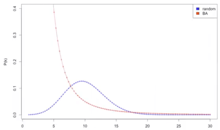
Cumulative function:
Distribution function:
m \Bigl ( \frac{t}{t_i} \Bigr )^{1/2} \leq k
P(k) = \frac{d F(k)}{dk} = \frac {2m^2}{k^3}
F(k) = P(k' \leq k) = \frac{n_0 + t - m^2t/k^2}{n_0 + t} \approx 1 - \frac{m^2}{k^2}
k_i(t) = m \Bigl ( \frac{t}{t_i} \Bigr )^{1/2}
Find probability \( P(k' \leq К) \) of a randomly selected node to have \( k \leq k \) at time \( t \) (fraction of nodes with \( k’ < k \) ). Nodes with \( k_i(t) \leq l \) :
t_i \geq \frac{m^2}{k^2} t
\longrightarrow
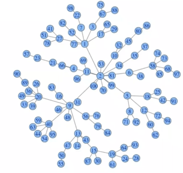
Preferential attachment model
Preferential attachment model
Preferential attachment model
Preferential attachment model
m = 1
m = 2
m = 3
Preferential attachment model
1. Growth
Node degree distribution function:
k_i(t) = m (1 + log(\frac{t}{i}))
P(k) = \frac{e}{m}exp(-\frac{k}{m})
П(k_i) =\frac{1}{n_0 + t + 1}
Node degree growth:
At each time step add a new node with \( m \) edges \( (m \leq n_0) \) ,
connecting to т nodes already in network \(k_i(i) = m \)
2. Attachment uniformly at random
The probability of linking to existing node \( i \) is
Preferential attachment model
Power law distribution function:
Clustering coefficient (numerical result):
< L > \sim \frac{log(N)}{log(log(N))}
P(k) = \frac {2m^2}{k^3}
Average path length (analytical result) :
C \sim N^{-0.75}
Preferential attachment model
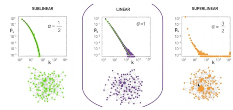
Non-linear preferential attachment models:
П(k) \sim k^{\alpha}
\( \alpha = 0 \) , no hubs, exponential dsitribution
\( 0 < \alpha < 1 \), sublinear, smaller hubs, stretched exponential
\( \alpha = 1 \) , scale-free, hubs, power law
\( \alpha > 1 \), superlinear, super hubs, hubs-and-spoke
Historical note
- Polya urn model, George Polya, 1923
- Yule process, Udny Yule, 1925
- Distribution of wealth, Herbert Simon, 1955
- Evolution of citation networks, cumulative advantage, Derek de Solla Price, 1976
- Preferential attachment network model, Barabasi and Albert, 1999
Local random models vs global optimization models
Network models
Empirical Network Features
- Power-law (heavy-tailed) degree destribution
- Small average distance (graph diameter)
- Large clustering coefficient (transitivity)
- Giant connected component, hierachical structure,etc
Generative models
- Random graph model (Erdos & Renyi, 1959)
- Preferential attachement model (Barabasi & Albert, 1999)
- Small world model (Watts & Strogatz, 1998)
G(n, p) Model
In the \( G(n, p) \) model, a graph is constructed by connecting nodes randomly. Each edge is included in the graph with probability \( p \) independent from every other edge. Equivalently, all graphs with \( n \) nodes and \( m \) edges have equal probability of \( p^m(1-p)^{(\frac{n}{2}-m)} \)
Erdos and Renyi, 1959.
\langle m \rangle = p \frac{n(n − 1)}{2}
\( G_{n,p} \) , each pair out of \( n(n − 1)/2 \) pairs of nodes is connected with probability \( p \), \( m \) - random number, \( \langle k \rangle \) - average node degree
\langle k \rangle = \frac{1}{n} \sum_i{k_i}=\frac{2 m }{n}=p(n-1) \approx pn
G(n, p) Model
Probability that \( i \) -th node has a degree \( k_i = k \)
(Bernoulli distribution)
- \( p^k \) - probability that connects to k nodes (has k-edges)
- \( (1 − p)^{n−k−1} \) - probability that does not connect to any other node
- \( C^k_{n-1} \) - number of ways to select k nodes out of all to connect to
P(k_i = k) = P(k) = C^k_{n-1}p^k(1-p)^{n-1-k}
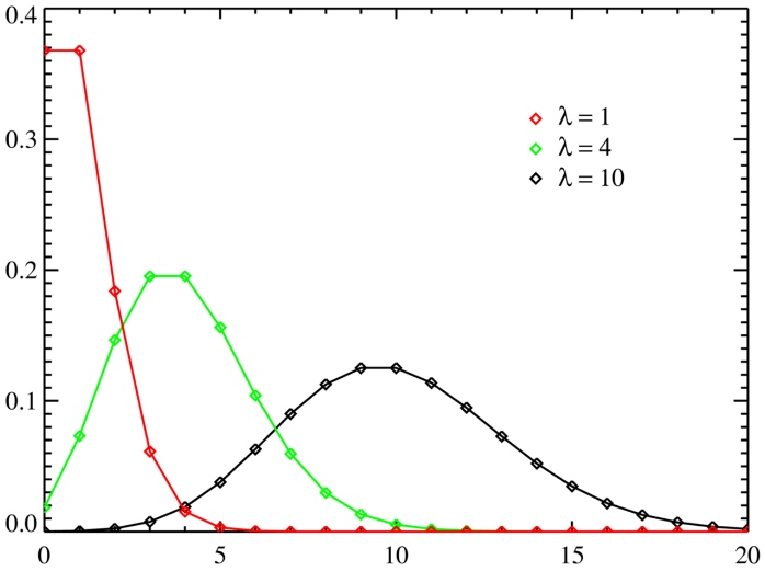
Limiting case of Bernoulli distribution, when \( n → ∞ \) at fixed \( \langle k \rangle = pn = λ \) (see upper formula)
P(k) = \frac{\langle k \rangle^ke^{-\langle k \rangle}}{k!}=\frac{λ^ke^{-λ}}{k!}
G(n, p) Model
Poisson distribution
Phase Transition
Consider \( G_{n,p} \) as a function of \( p \)
- \( p = 0 \), empty graph
- \( p = 1 \), complete (full) graph
- There are exist critical \( p_c \) , structural changes from \( p < p_c \) to \( p > p_c \)
- Gigantic connected component appears at \( p > p_c \)
Let \( u \) - fraction of nodes that do not belong to GCC. The probability that a node does not belong to GCC
u = p(k=1)•u + P(k=2)•u^2 + P(k=3)•u^3 ... =
= \sum_{k=0}^∞{P(k)u^k} = \sum_{k=0}^∞ \frac{λ^ke^-λ}{k!}= e^{-λ}e^{λu} = e^{λ(u-1)}
Phase Transition
Let \( s \) -fraction of nodes belonging to GCC (size of GCC)
- when \( λ \rightarrow ∞, s \rightarrow 1 \)
- when \( λ \rightarrow 0, s \rightarrow 0 \)
- \( λ=pn \)
s = 1 — u
1-s=e^{-λs}
- \( λ_c = p_cn = 1 \)
- \( p_c = \frac{1}{n} \)
Small world model
Threshold probabilities when different subgraphs of g-nodes appear in a random graph
- \( p_c \sim n^{-g/(g-1)} \) having a tree of order \( g \)
- \( p_c \sim n^{-1} \), having a cycle of order \( g \)
- \( p_c \sim n^{-2/(g-1)} \) complete subgraph of order \( g \)
s = 1 — u
1-s=e^{-λs}
- \( λ_c = p_cn = 1 \)
- \( p_c = \frac{1}{n} \)
03-2
Small world
Small world model
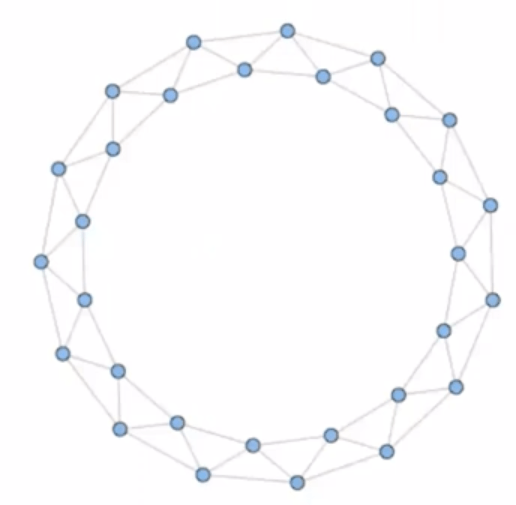
Motivation: keep high clustering, get small diameter
Clustering coefficient С = 1/2
Graph diameterd = 8
Small world model
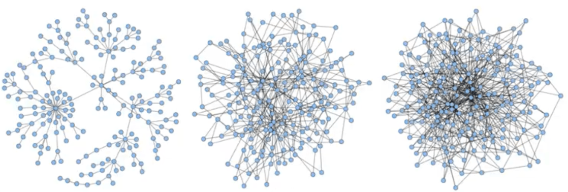
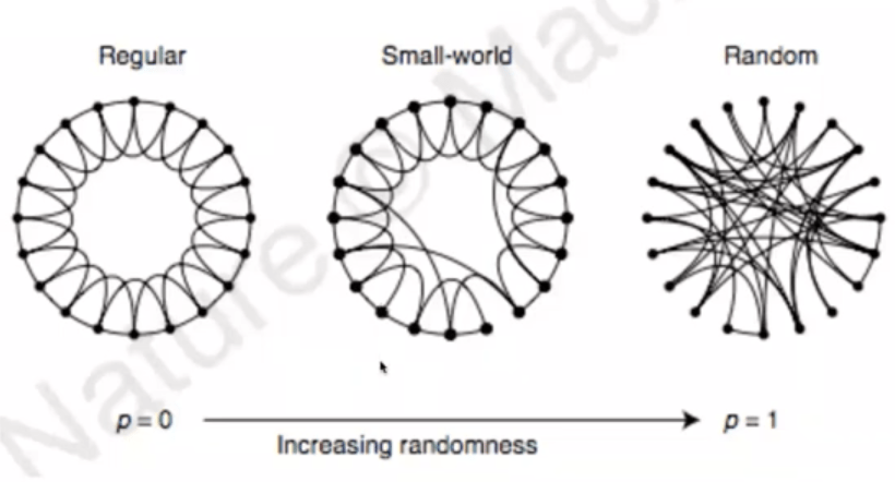
Single parameter model, interpolation between regular lattice and random graph
- start with regular lattice with п nodes, К edges per vertex (node degree), \( k << n \)
- randomly connect with other nodes with probability р, forms \( pnk/2 \) "long distance” connections from total of \( nk/2 \) edges
- \( р = 0 \) regular lattice, \( р = 1 \) random graph
Watts and Strogatz, 1998
Small world model
Small world model
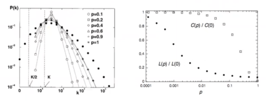
Node degree distribution:
Poisson like
Ave. path length \( \langle L(p) \rangle \) :
\( р \longrightarrow 0 \) , ring lattice, \( \langle L(p) \rangle = n/2k \)
\( р \longrightarrow 1 \) , random graph, \( \langle L(p) \rangle = log(n)/log(k) \)
Clustering coefficient C(p) :
\( р \longrightarrow 0 \) , ring lattice, C(0) = 3/4 = const
\( р \longrightarrow 1 \) , random graph, С(1) = k/n
Small world model
Model comparison
| Random | BA | WS | Empiracal nets | |
|---|---|---|---|---|
|
|
poisson like | power law | ||
|
|
const | large | ||
|
|
small |
\frac{\lambda^k e^{-\lambda}}{k!}
\langle k \rangle / N
\frac{log(N)}{log(\langle k \rangle)}
\frac{log(N)}{log(log(\langle k \rangle))}
log(N)
k^{-3}
N^{-0.75}
P(k)
\langle L \rangle
C
Network Models
By karpovilia


