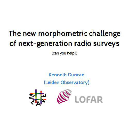
Optimizing photometric redshifts for LOFAR sources
Kenneth Duncan
LOFAR Meeting - Bologna, Sept 2016
Leiden Observatory
Optical photometry across the LOFAR Tier 2 & 3 fields
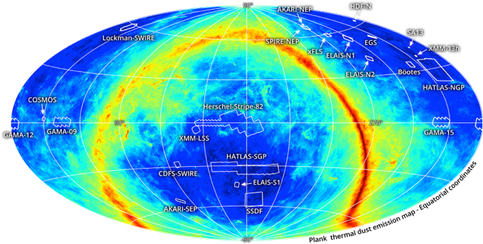
Close collaboration with HELP (Herschel Extragalactic Legacy Project - PI S. Oliver)
Collecting and matching all publicly available imaging
Will include photometric redshifts and multi-wavelength physical modelling for all Herschel fields
Optical photometry across the LOFAR Tier 1
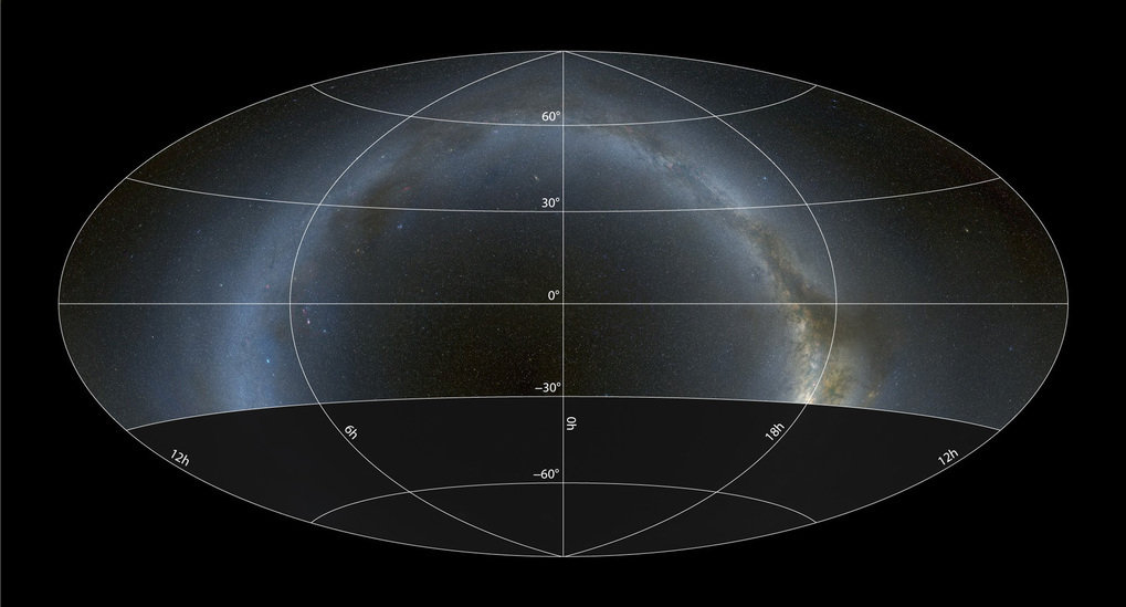
'All sky'
PanSTARRS optical (grizy)
UKIRT Hemisphere near-IR (J)
WISE mid-IR (3.4um/4.5um)
PanSTARRs 3pi survey coverage
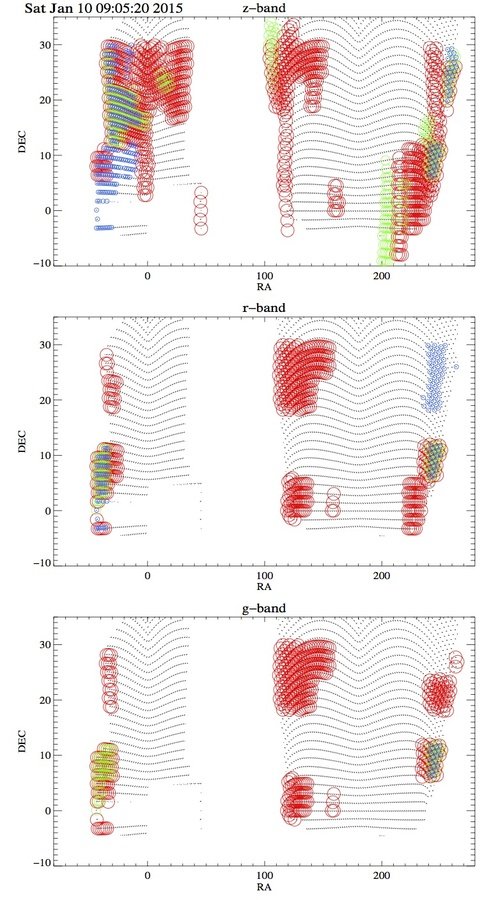
Deeper patches
DECALS: -20° < δ < +30°
HyperSuprimeCam Survey
Template fitting photo-z estimates
Step 1: The code
EAZY
Brammer et al. (2008)
LePhare
Arnouts et al. (1999)
Ilbert et al. (2006)
PhotoZ
Bender et al. (2001)
Hyper-Z
Bolzonella et al. (2000)
ZEBRA
Feldmann et al. (2006)
BPZ
Benitez (2000)
Step 1: The code
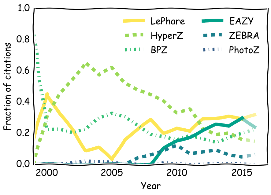
Total citations: ~2800
Then
Now
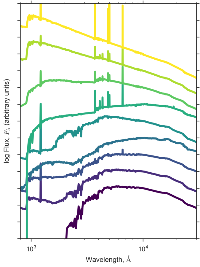
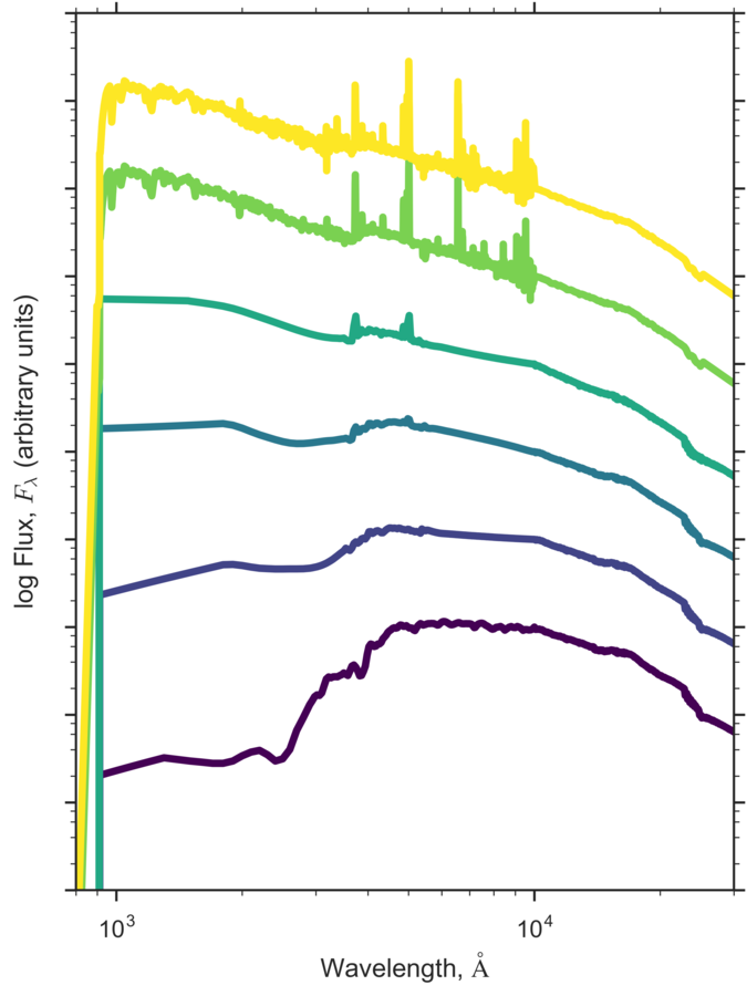
Step 2: The Templates
Step 3: zeropoint offsets and additional smoothing errors
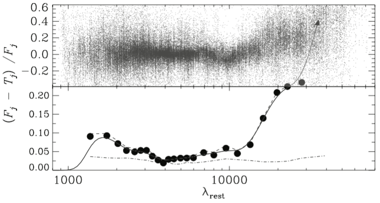
Additional rest-frame errors
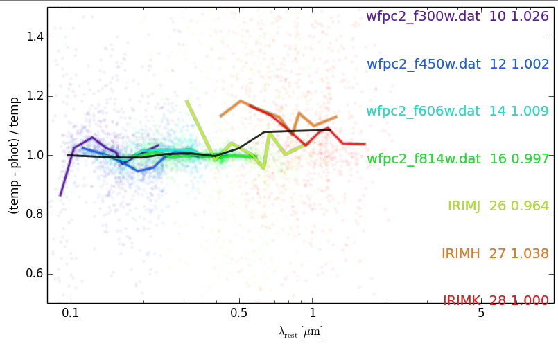
Corrections to the observed zeropoints
Brammer et al. (2008)
Dust
AGB Stars?
PAH/Dust emission/AGN?
Step 4: priors (optional)
Brammer et al. (2008)
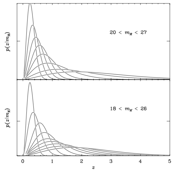
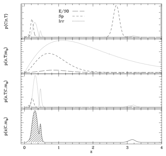
Benitez (2000)
Magnitude
Spectral type
Training based photo-z estimates
(aka machine learning)
Aside: Motivations for ML-based Photo-z's
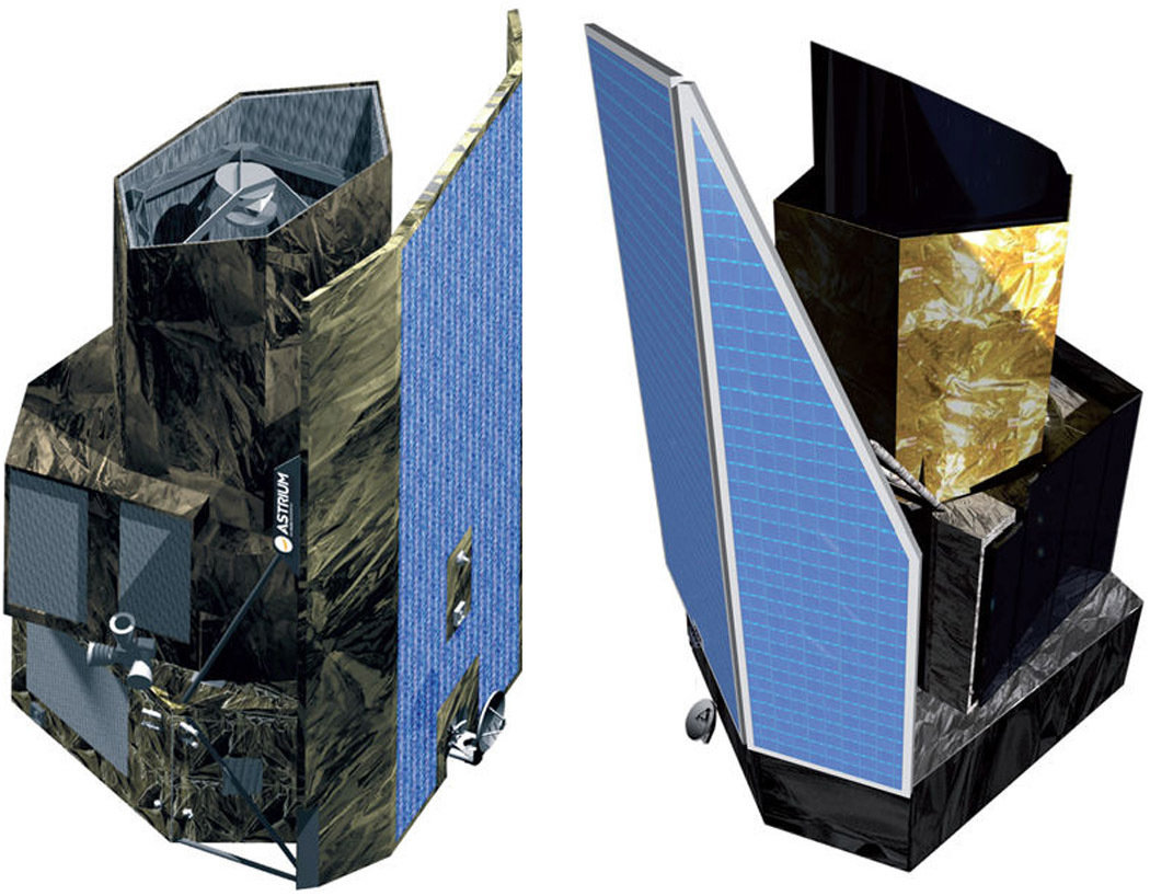
Euclid
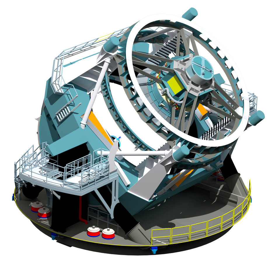
LSST
Aside: Motivations for training (ML) based Photo-z's
1. Speed
Euclid: ~1.5 billion galaxies
LSST: ~10 billion galaxies
Estimated time to run EAZY on all sources (on a desktop machine):
~2+ years (Euclid)
~14+ years (LSST)
Motivations for training (ML) based Photo-z's
2. Improvements in accuracy
Sanchez et al. (2014)
Weak Lensing requirements:
Scatter
\sigma_{z}/(1+z) < 5\%
\langle z \rangle / (1+z) < 0.2\%
Bias
Step 1: Select your training sample
i.e. a representative subset of your sample with spectroscopic redshifts
Step 2: Pick your favourite regression/classification algorithm
Neural Networks
Self-organizing Maps (SOMs)
Deep learning
Support Vector Machines (SVM)
Naive Bayes
Gaussian Processes
Generalized Linear Models
Bayesian Network
k-Nearest Neighbour
Boosted Decision Trees
Randomised Forests
Relevance vector machines
Radial basis function networks
Normalised inner product nearest neighbour
Directional neighbourhood fitting
Voronoi tesselation density estimator
Non-conditional density estimation
Step 3: Train your regression/classification algorithm
Step 4: Apply to your science sample
magic happens somewhere here
Pros and Cons of ML Photo-z's
Pro:
- Fast and scalable
- Entirely empirical:
no concern about template choice
- Simple to include extra information:
properties such as size and morphology can help break degeneracies
Con:
- Entirely dependent on spectroscopic training sample
- Struggle more with inhomogeneous datasets (e.g. missing filters)
- Difficult to physically interpret solutions - e.g. rest-frame colours
Final step: (For all photo-z methods)
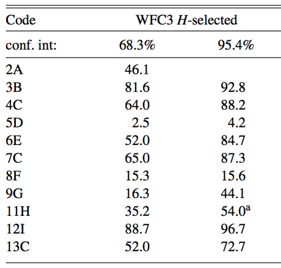
Fraction of spectroscopic redshifts within given confidence interval
Dahlen et al. (2012)
!
7/11 submitted photo-z estimates significantly overconfident for 1-sigma errors
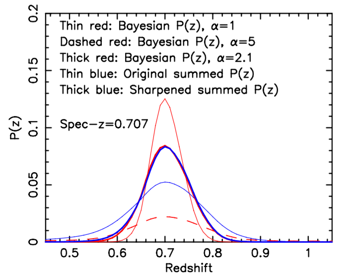
Calibrating redshift pdfs
Calibrating redshift pdfs
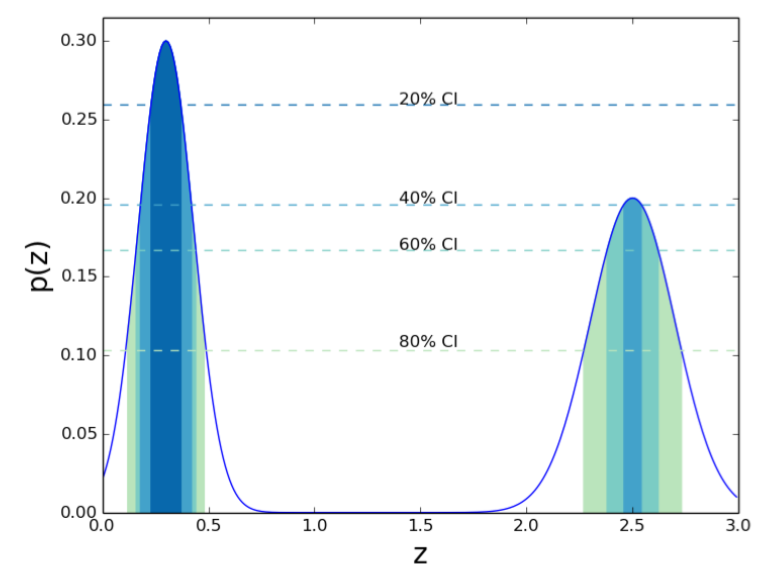
Wittman et al. (2016)
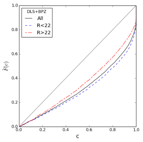
See also Bordoloi et al. (2010)
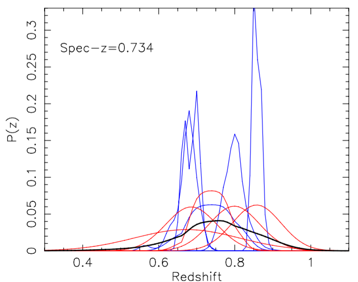
Improving photo-z estimates even more...
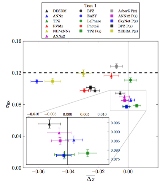
the wisdom of crowds
Combine multiple photo-z estimates
Dahlen et al. (2012)
= Median of all photo-z estimates
= Median of best 5 photo-z estimates
See also Carrasco Kind & Brunner (2014)
Also works for diff. templates with the same code
Limits of existing spectroscopic samples
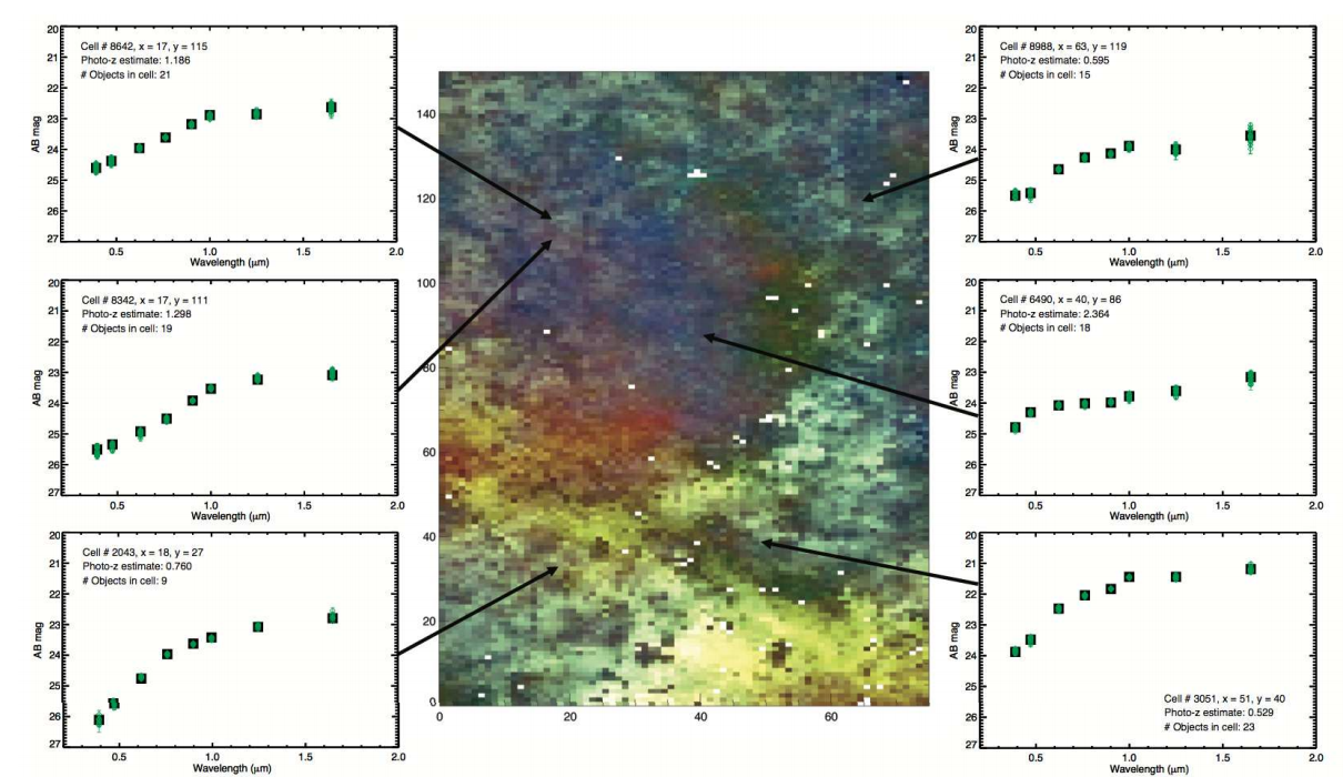
Masters et al. (2015)
Limits of existing spectroscopic samples
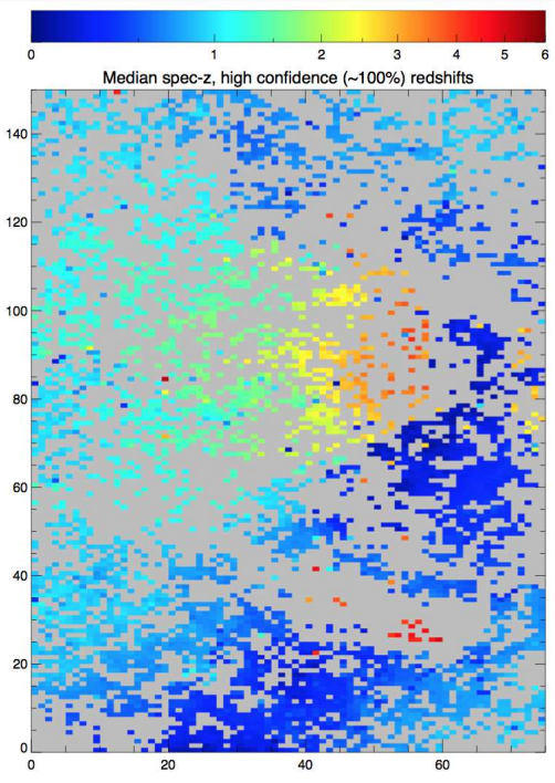
Masters et al. (2015)
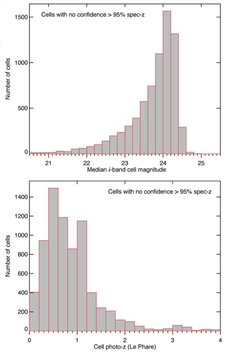
Limits of existing spectroscopic samples
Masters et al. (2015)
Short term solution:
Targeted spectroscopic follow-up of unexplored colour space (Underway): ~< 10k spectra
Ongoing spectroscopic surveys:
(e.g. VANDELS/HETDEX)
Long term solution (2018+):
New massively multiplexed spectroscopic surveys -
Subaru/PFS and WHT/WEAVE in the North: ~1m+ spectra
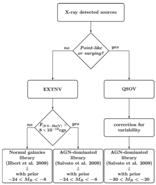
Example: Phot-z's for X-ray Sources
Faint X-ray sources better fit by 'normal' galaxies
Salvato et al. (2009/11)
Redshifts for LOFAR sources
Suggested strategy...
* Carrasco Kind and Brunner (2014)
Bayesian model combination/averaging (BMC/BMA)*
Test field
Spectroscopic sample (Bootes)
N x Photo-z estimates
e.g.:
AGN/QSO Templates
Stellar Templates
(ML estimates)
Photo-z's Optimised for all source types a priori
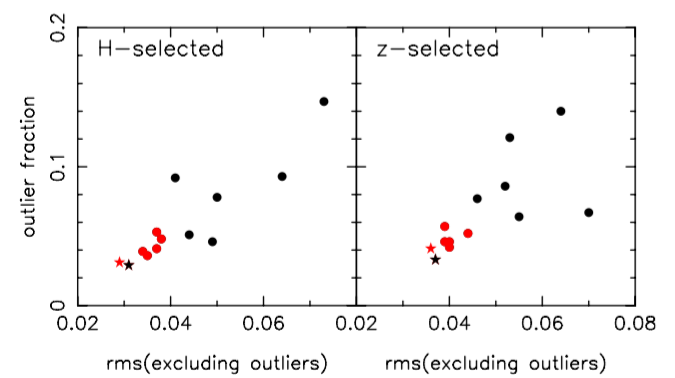
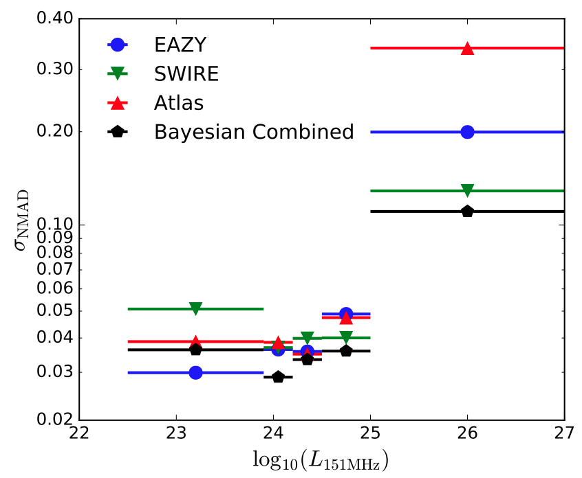
Q. How good will the redshifts for LOFAR sources be?
Q. How good will the redshifts for LOFAR sources be?
Q. How good will the redshifts for LOFAR sources be relative to non-radio sources?
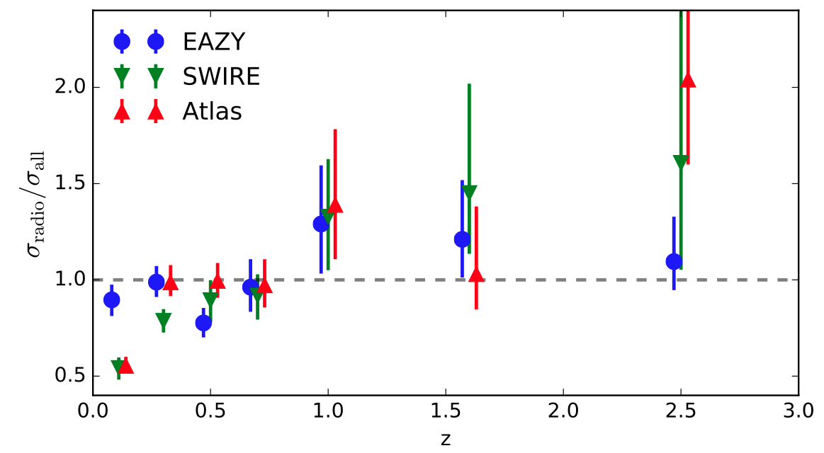
EAZY
SWIRE
'Atlas'
Stellar only
Stellar + AGN
Stellar + AGN
Duncan et al. (in prep)
EAZY
SWIRE
'Atlas'
Stellar only
Stellar + AGN
Stellar + AGN
Duncan et al. (in prep)
Fixed redshift bin
0.4 < z < 0.8
Summary: what to expect in future
1. Full multi-wavelength optical photometry in Tier-2/Tier-3 fields will be available through HELP
2. Optimised photometric redshifts will also be available as and when each field is completed by HELP
3. For all but the highest luminosity sources, photo-z accuracy should be comparable to normal galaxies (more work required)
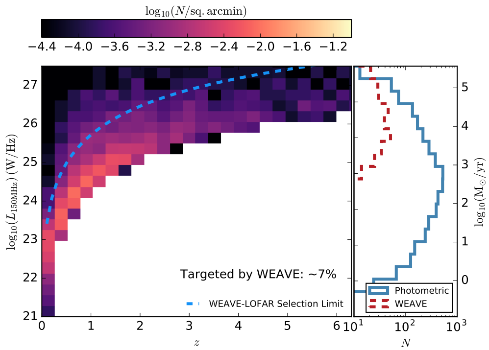
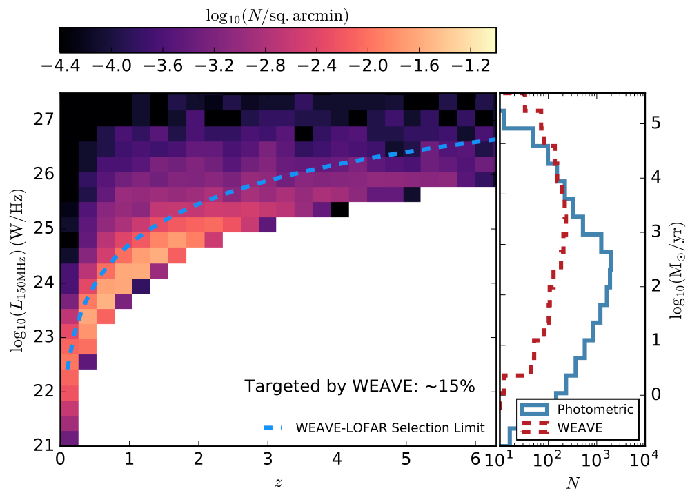
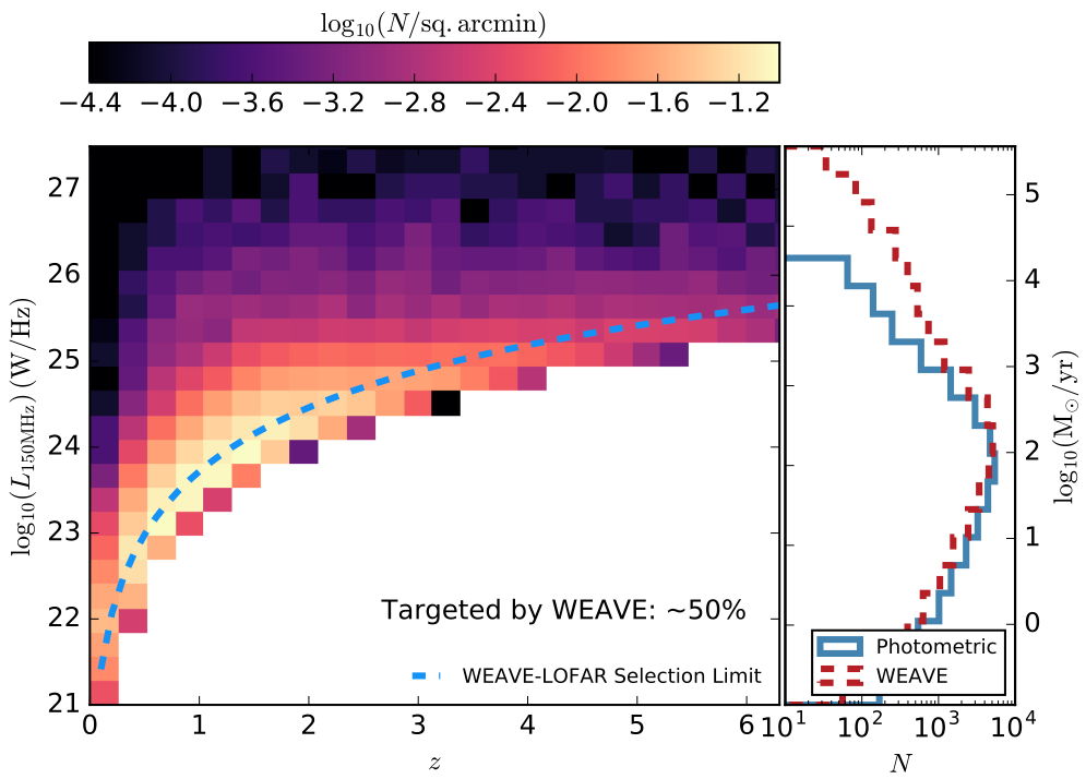
But...these luminous sources will be targeted by WEAVE
Photometric redshifts for LOFAR
By Kenneth Duncan
Photometric redshifts for LOFAR
Review of photometric redshifts past, present and future. For the Lorentz Workshop Jun 20th-24th