From random forests to regulation: interpreting supervised learners to guide biological discovery
Karl Kumbier
December 16, 2020
In search of mechanistic insights into development and function

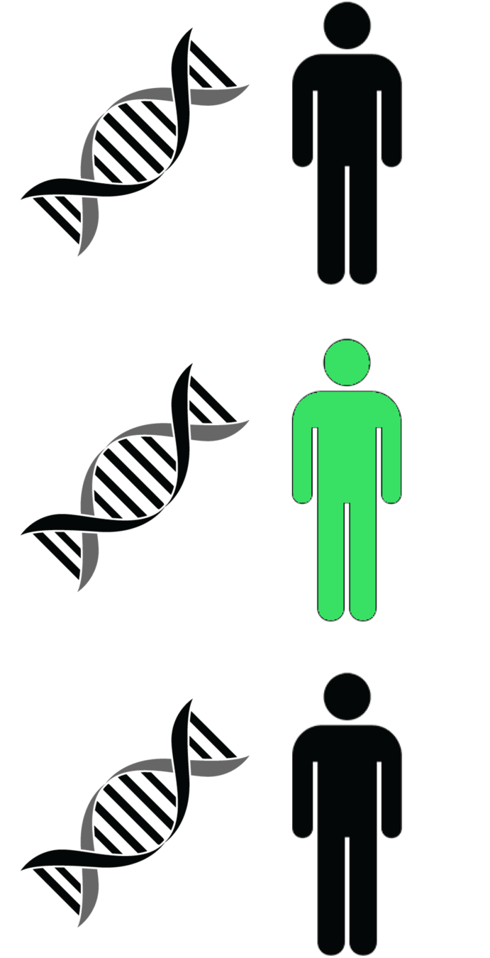
- Genomes contain vast amounts of information (e.g. 6M variants in 20K human genes)
- Complex biological processes are the result of interacting components
- Linking genomic processes to biological outcomes requires the exploration of enormous spaces
Domain insights through supervised learning
Natural phenomena
ML models
Domain insights
?
Prediction
Interpretation
"Accuracy generally requires more complex prediction methods."
- Leo Breiman, Statistical Modeling: The Two Cultures (2001)
Outline
-
From genomic to statistical interactions
-
Market baskets and genomics
-
Iterative random forests & signed iterative random forests
-
Case studies: Interaction discovery in Drosophila and UK Biobank cohort
From genomic to statistical interactions
Embryonic development in Drosophila
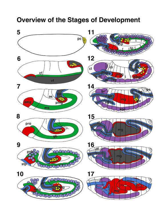


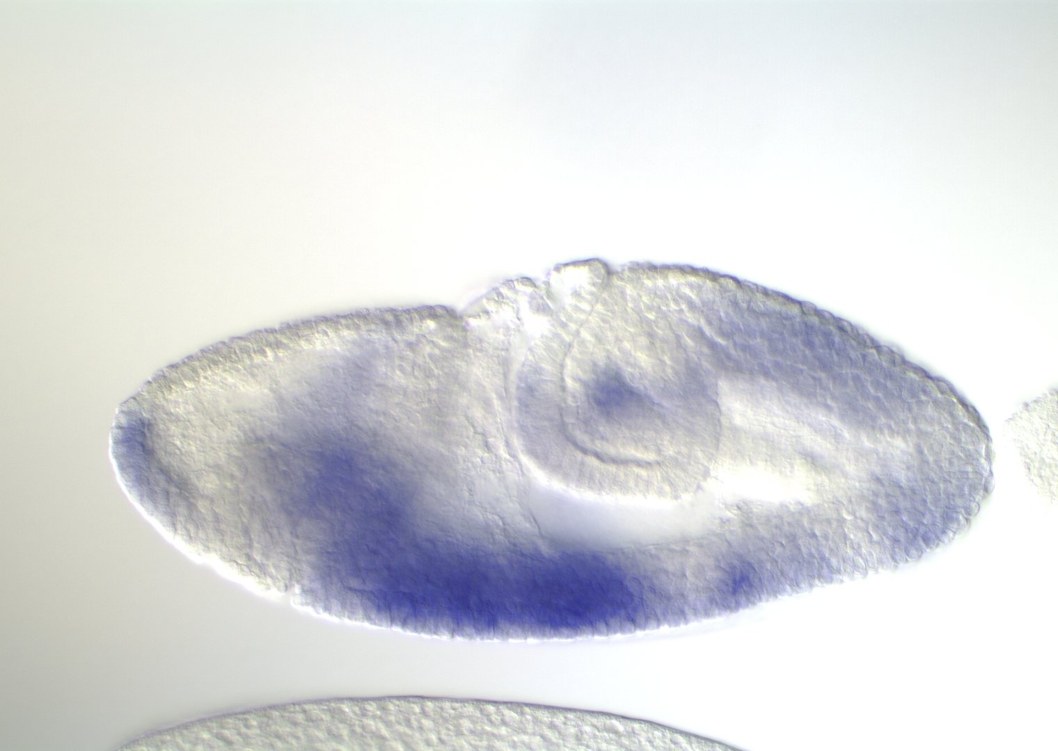

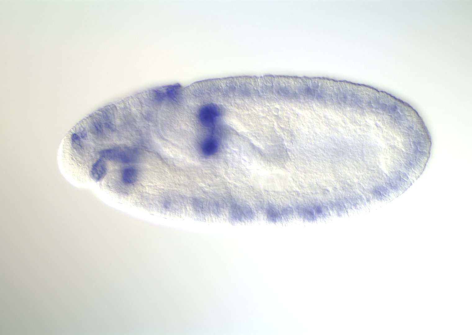
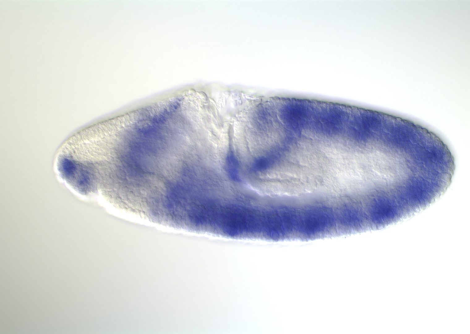
0-1:20 hours
1:20-3:00 hours
3:00-3:40 hours
3:40-5:20 hours
5:20-9:00 hours
9:20-16:00 hours
image: Volker Hartenstein
images: BDGP
Kr expression
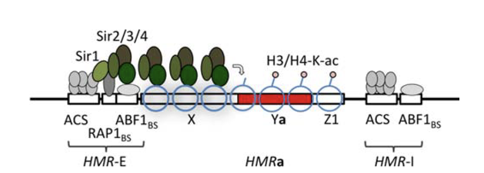
Enhancers regulate spatio-temporal programs of gene expression
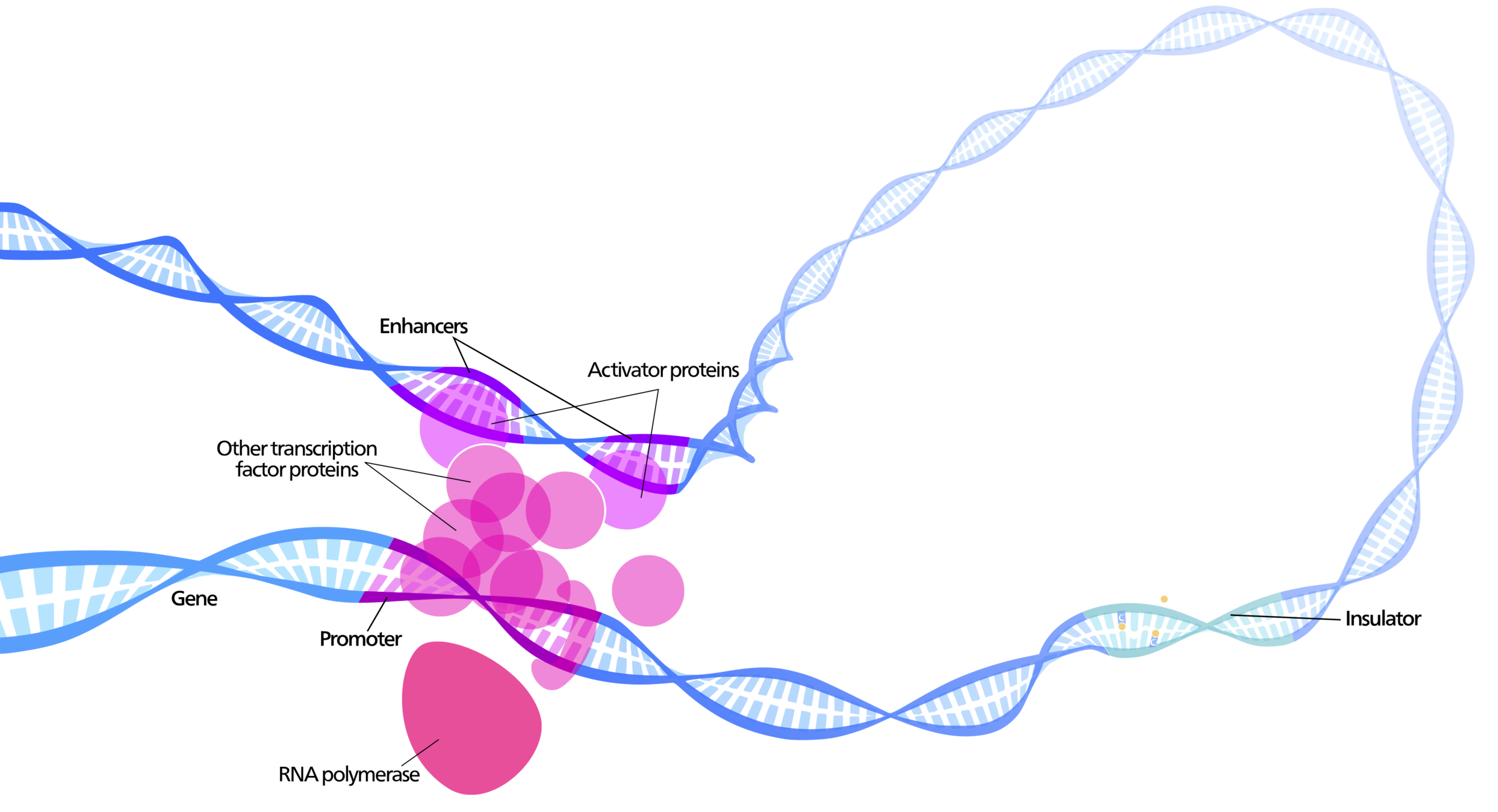
Enhancers: segments of the genome that coordinate transcription factor (TF) activity to regulate gene expression.
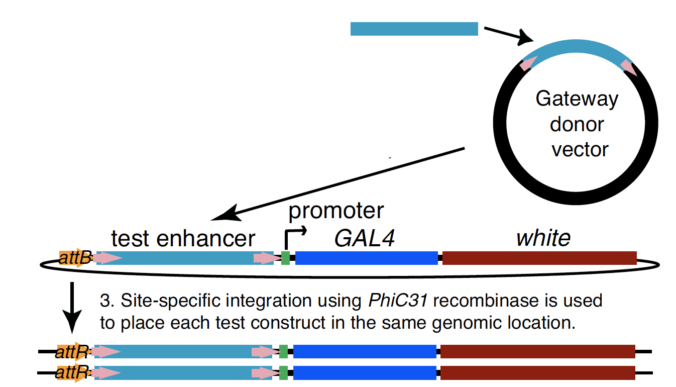
Experimental evaluation of enhancer elements in Drosophila
Pfeiffer et al. (2008)
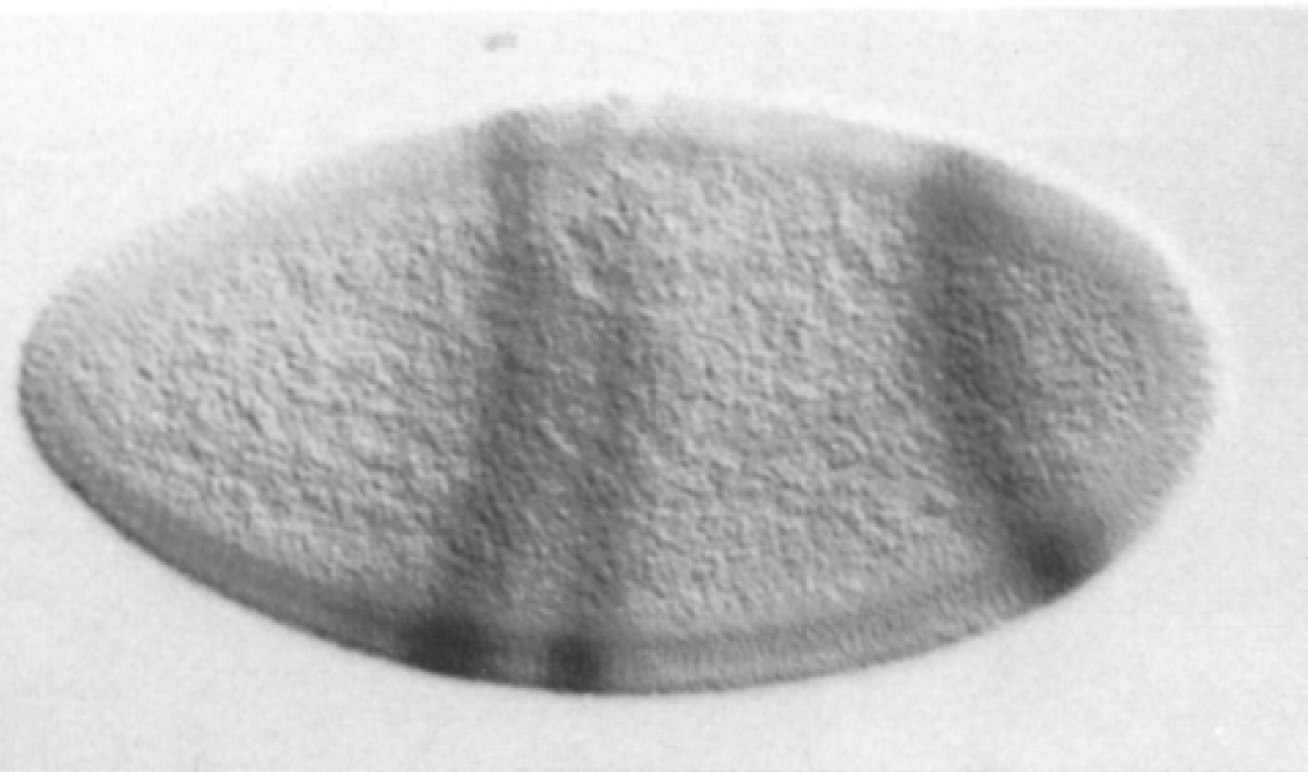
even-skipped
expression
wt
transgenic
Experimental evaluation of enhancer elements in Drosophila
Hiromi et al. (1985), Harding et al. (1989), Goto et al. (1989), Pfeiffer et al. (2008)
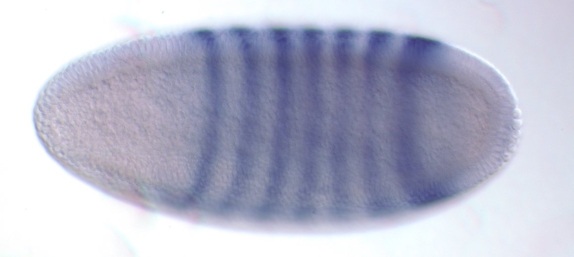
even-skipped expression
wt
transgenic
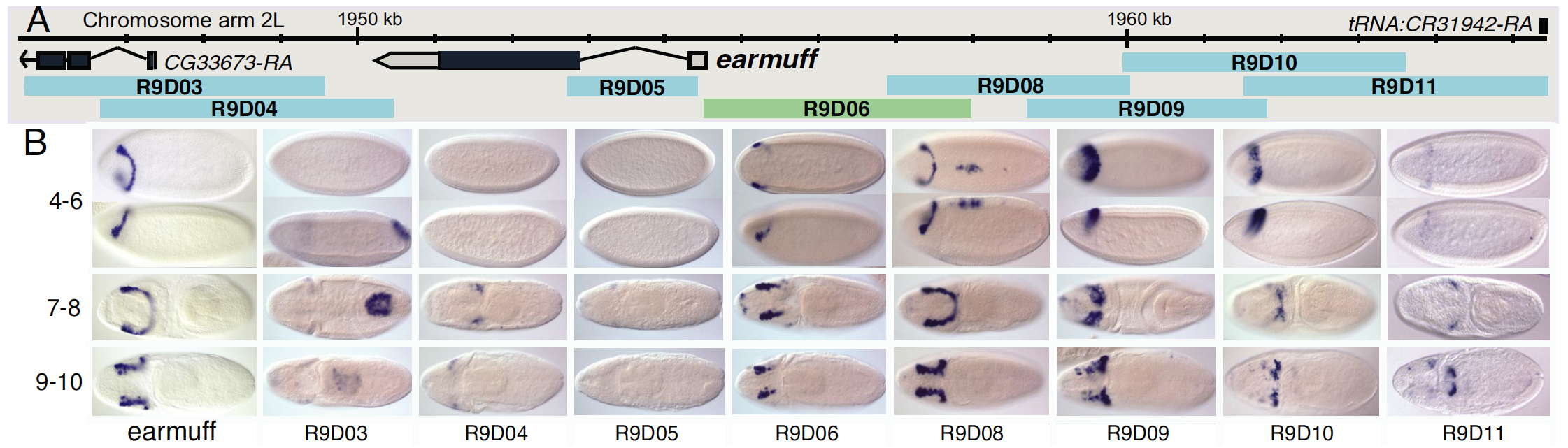
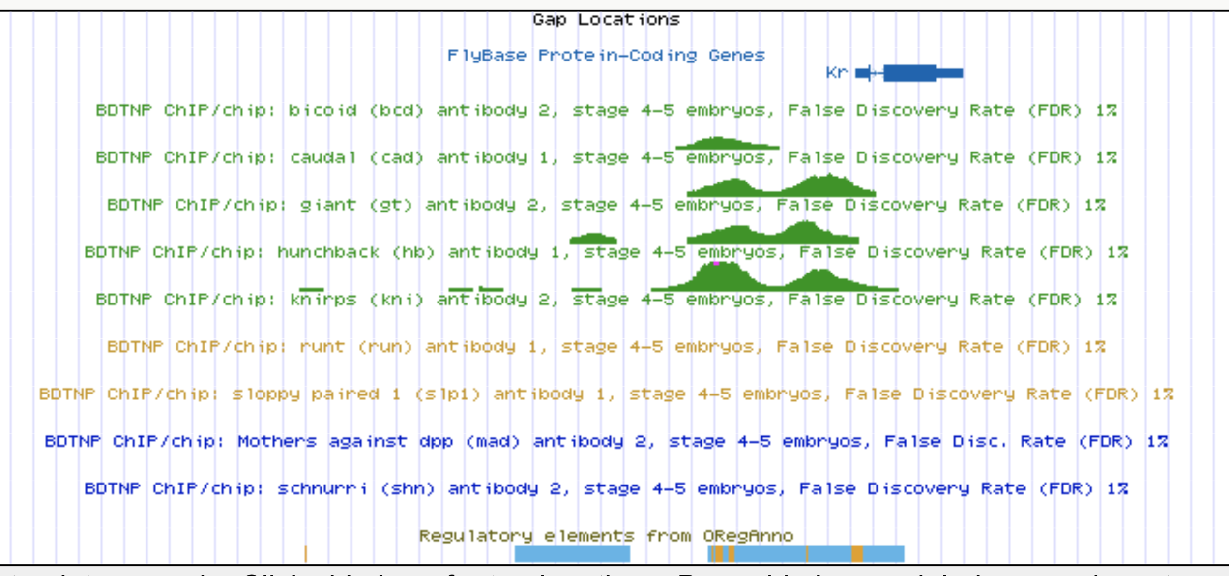
Identifying regulatory interactions from high-throughput genomic data
Experimentally validated enhancer elements.
Whole-embryo ChIP-chip/ChIP-seq measurements of transcription factor (TF) DNA binding

- Fisher (epistasis): "deviation from the addition of superimposed effects (...) between different Mendelian factors."
- Traditionally formulated as a multiplicative interaction term (e.g. in logistic regression)
From genomic to statistical interactions: classical interpretation
logit(p) = \beta_0 + \beta_1 x_1 + \beta_2 x_2 + \beta_{12} x_1 x_2
Problems
- Non additivity depends on response scaling
- Computationally intractable for high-order interactions
- TF interactions are not necessarily multiplicative
High-order interactions at enhancer elements drive embryonic development
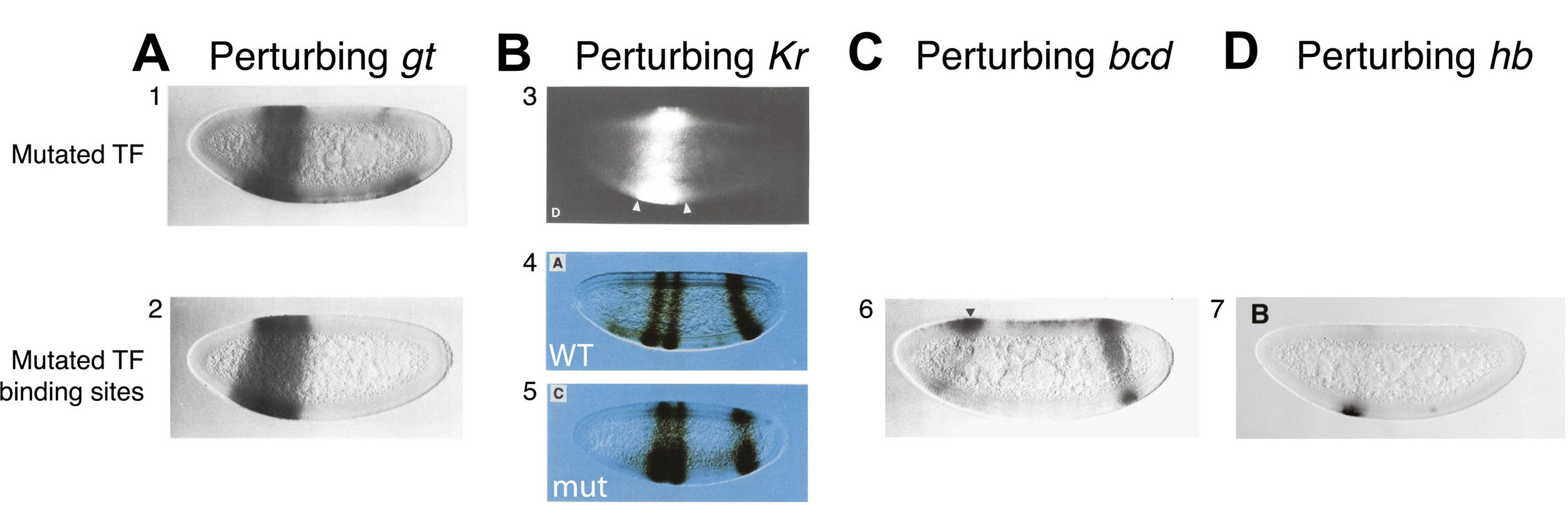
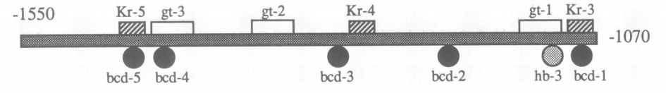
Goto et al. (1989), Harding et al. (1989), Small et al. (1992), Isley et al. (2013), Levine et al. (2013)
From genomic to statistical interactions: our interpretation
r(\mathbf{x})=
\prod_{j\in\text{A}} 1(x_j > t_j)
\cdot
\prod_{j\in\text{R}} 1(x_j \le t_j)
activators
repressors
\mathbf{x}=(x_1, \dots, x_p)
Segment of the genome
DNA binding for p transcription factors (TFs)
Order-s interaction: s = #activators + #repressors
r(\mathbf{x}) = 1
x_{bcd}
x_{cad}
\dots

RuleFit: rule-based interaction discovery (Friedman and Popescu, 2008)
- Identify a collection of marginally important features
- Search for predictive order-2 rules among marginally important features
\dots
Computational costs grow as
O(p^s)
Misses interactions with weak marginal effects
image: Lee and Haber (2014)
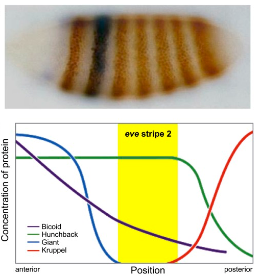
Thresholding rules define expression domains
Chopra and Levine (2009)
Dl +
Dl -
Wolpert (1968), Jaeger and Reinitz (2006), Chopra and Levine (2009), Zizen et al. (2009), Knowles and Biggin (2013), Levine (2013), Staller al. (2015), ...
Jaeger and Reinitz (2009)
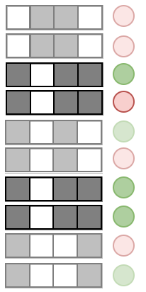
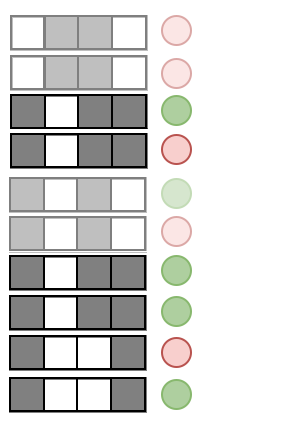
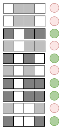
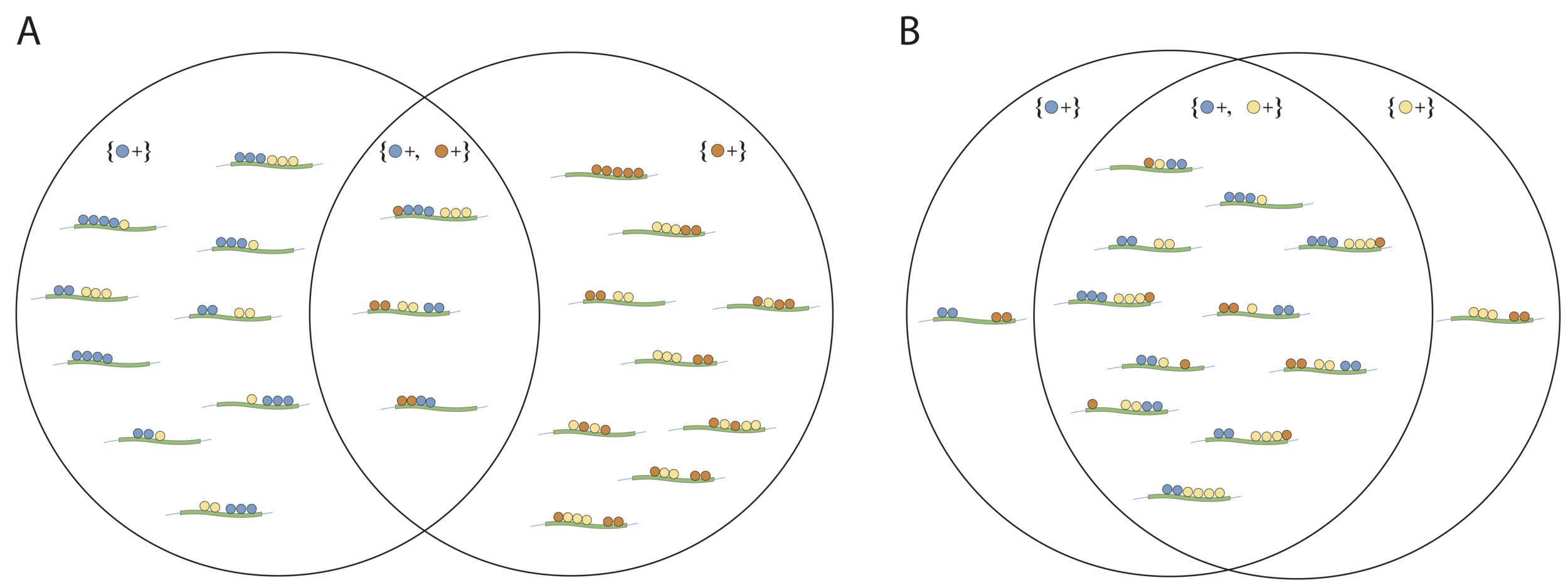
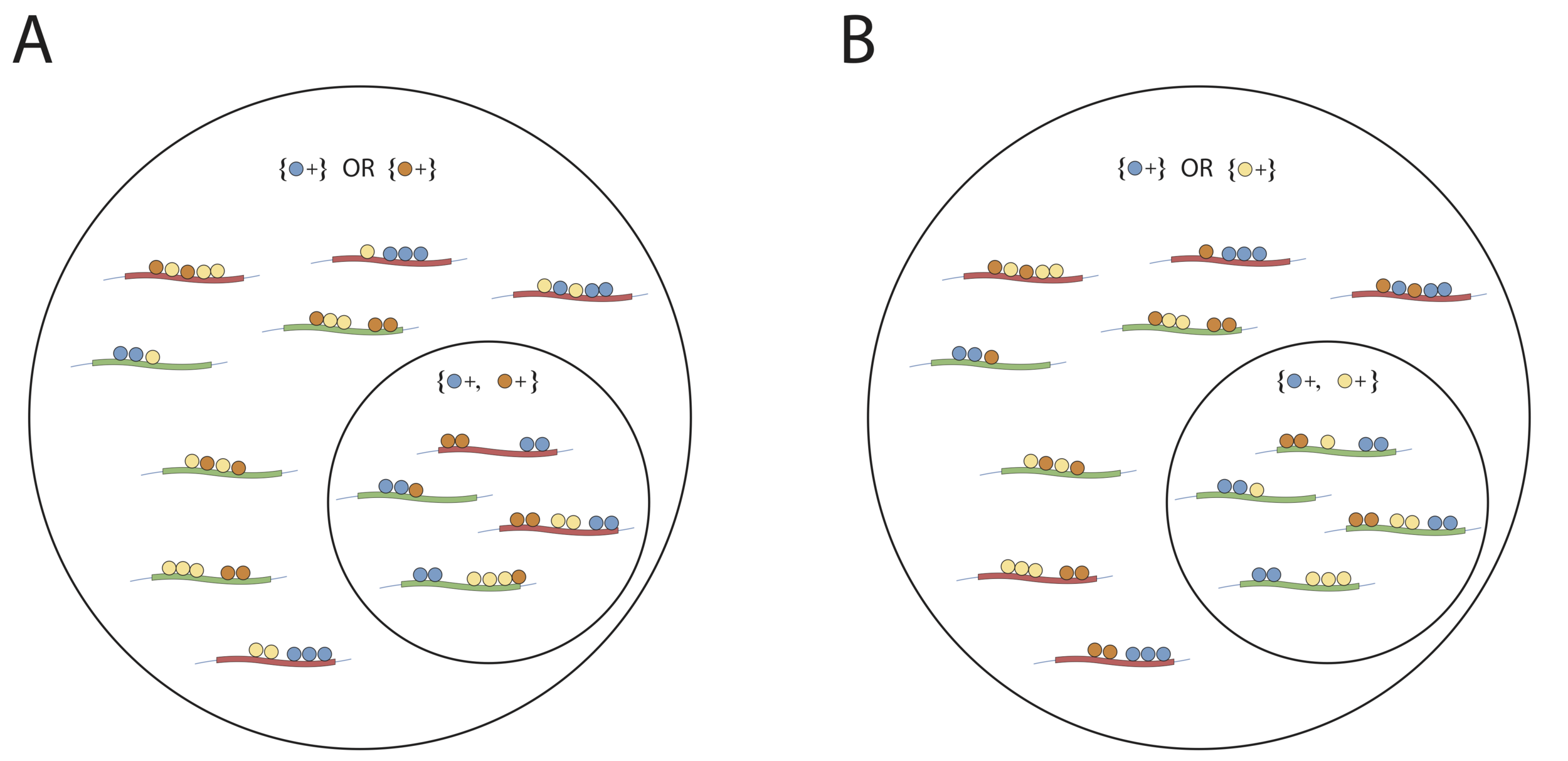
From genomic to statistical interactions
\mathbb{P}_n(y = 1 | S)
\mathbb{P}_n(S|y = 1)
(1) How precisely does an interaction predict class-1 observations?
(2) How prevalent is an interaction among class-1 observations?
S = (x_{j_1} > t_{j_1}) \,\&\, \dots \,\&\, (x_{j_s} \le t_{j_s})
Interactions:
Responses:
y \in \{0, 1\}
r(\mathbf{x})=
?
Market baskets and genomics
Interactions in market baskets


What combinations of items do customers purchase together?
Interactions in market baskets
What combinations of items do customers purchase together?
What combinations of items do different types of customers purchase together?


Interactions in market baskets
Z_1
Z_2
Z_3
Z_4
\mathcal{I}_1
\mathcal{I}_2
\mathcal{I}_3
\mathcal{I}_4
Feature-index sets
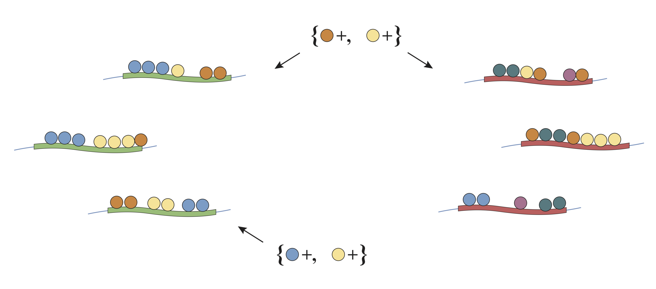
Random intersection trees (RIT)
Shah and Meinshausen (2014)
Leverage sparsity in market baskets to search for frequently co-occurring items in a computationally efficient manner
- Randomly sample feature index sets from class-C observations:
- Intersect sampled feature index sets in a tree like fashion up to depth D
- Return all feature combinations that "survive" intersection procedure up to depth D
\{\mathcal{I}_i \subseteq\{1, \dots, p\}: Z_i = C\}
Random intersection trees (RIT)
Shah and Meinshausen (2014)
Randomly sampled
class-C observation
"survived" interaction
Random intersection trees (RIT)
Shah and Meinshausen (2014)
Random intersection trees (RIT)
Shah and Meinshausen (2014)
Genomic response
Genomic features
Translating the market basket problem into genomics

\dots
Genomic response
Genomic features
Translating the market basket problem into genomics
Challenges:
- Genomic features are typically measured in concentrations/counts
- Binding does not imply regulation (Li et al. 2008)
\dots
iterative Random Forests (iRF)
&
signed iterative Random Forests (siRF)
Joint work with Sumanta Basu, James B. Brown, and Bin Yu


iterative Random Forest to identify high-order interactions in genomic data
- Iteratively re-weighted Random Forests stabilize decision path
- Generalized random intersection trees search for high-order interactions
- Stability bagging evaluates interactions
iterative Random Forests (iRF) build on predictability, computability, and stability to identify genomic interactions in developing Drosophila embryos
Open source R implementation: github.com/karlkumbier/iRF2.0
Iteratively re-weighted random forests
Classification and regression trees (CART)
Breiman et al. (1984)
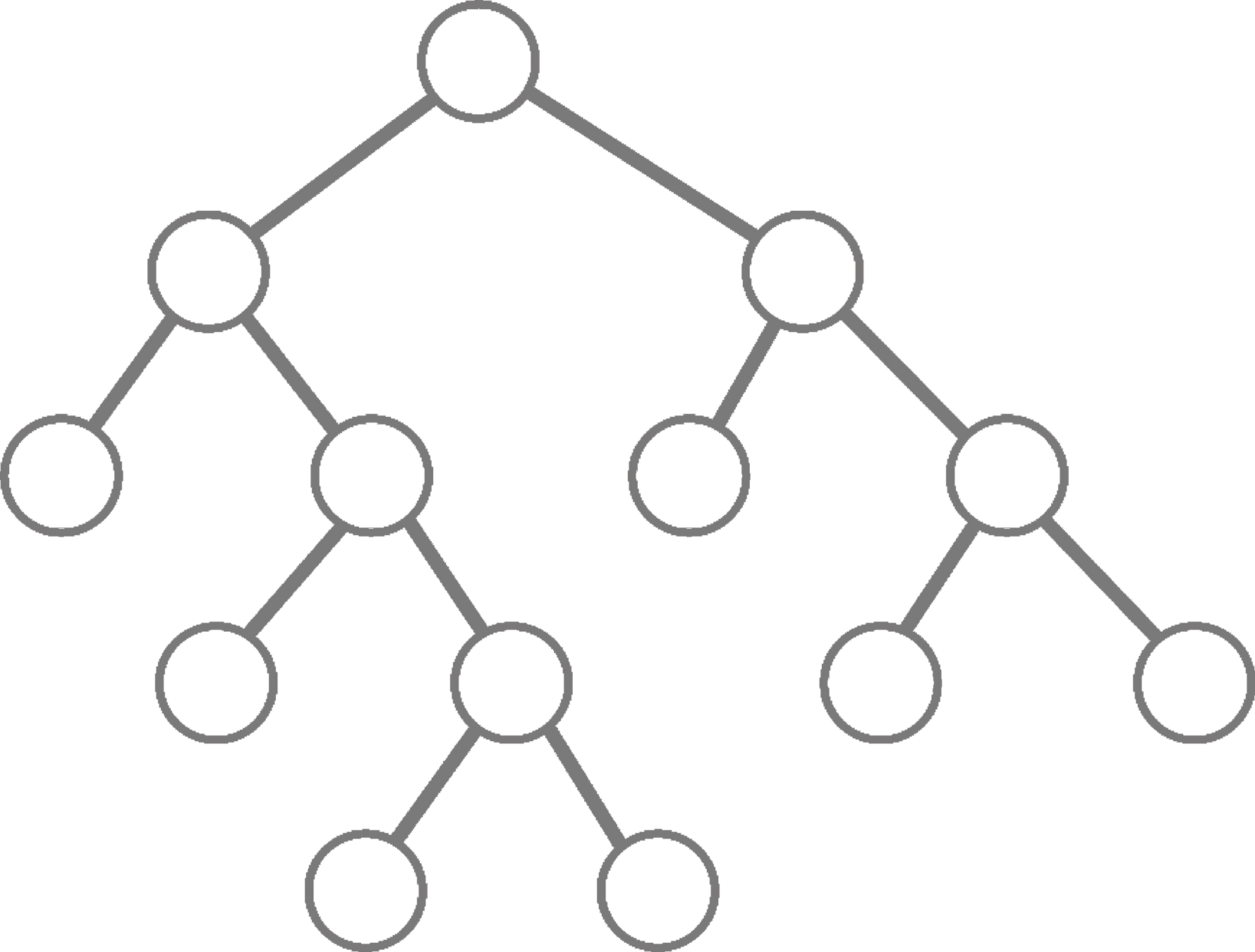
For current node:
- Select splitting feature and threshold
- Partition data
- Repeat until stopping criteria
x_2>t_2
x_3>t_3
x_4>t_4
Classification and regression trees (CART)
Breiman et al. (1984)
For current node:
- Select splitting feature and threshold
- Partition data
- Repeat until stopping criteria
x_2>t_2
x_3>t_3
x_4>t_4
(x_2 > t_2) \,\&\,(x_3 > t_3) \,\&\,(x_4 > t_4)
Random Forests
Breiman (2001)
Random forests modify CART to improve predictive accuracy:
- CART trees are trained on bootstrap samples of the data
- CART criterion evaluated on subset of features sampled uniformly at random
Random forest modifications improve generalization but reduce stability!
Feature-weighted Random Forests
Amaratunga et al. (2008)
Random forests:
At each node of the decision tree, uniformly sample a subset of features
Feature-weighted random forests:
At each node of the decision tree, sample a subset of features with probability proportional to
w\in\mathbb{R}^p_+
w_1
w_2
w_3
w_4
w_5
w_1
w_2
w_3
w_4
w_5
Feature weights
The CART criterion: Gini impurity
(\pi, N)
(\pi_l, N_l)
(\pi_r, N_r)
Proportion positive responses
Number of observations
Gini impurity:
I_G(\pi) = \pi (1-\pi)
Decrease in Gini impurity:
I_G(\pi)-\frac{N_l}{N}I_G(\pi_l) - \frac{N_r}{N}I_G(\pi_r)
Mean decrease in impurity:
On average, how much does splitting on a variable decrease the Gini impurity?
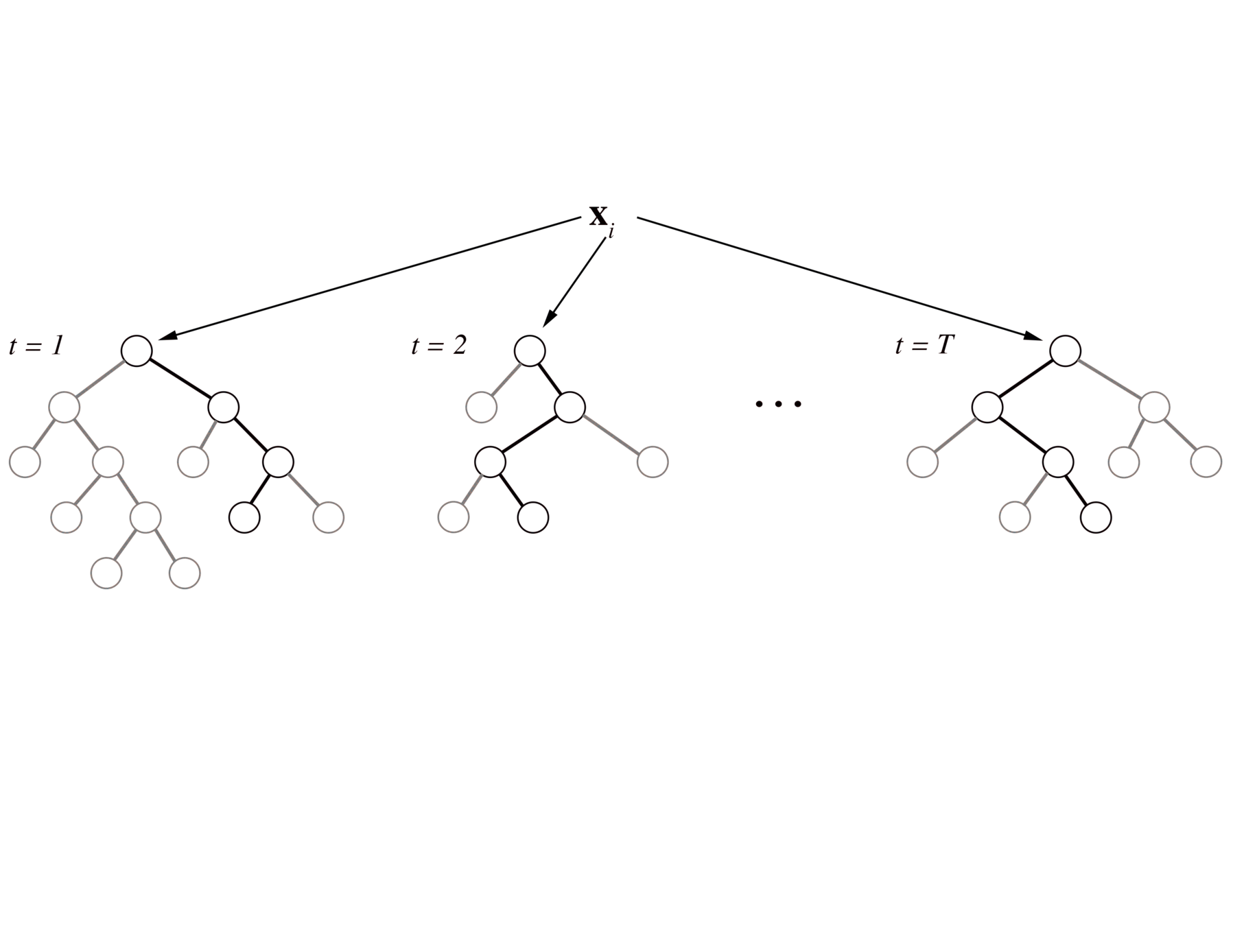
Iterative re-weighting stabilizes random forest decision paths
Gini importance
Iteration 1
Iteration K
w_1
w_2
w_3
w_4
w_5
w_1
w_2
w_3
w_4
w_5
Feature weights
Iterative re-weighting helps recover high-order interactions
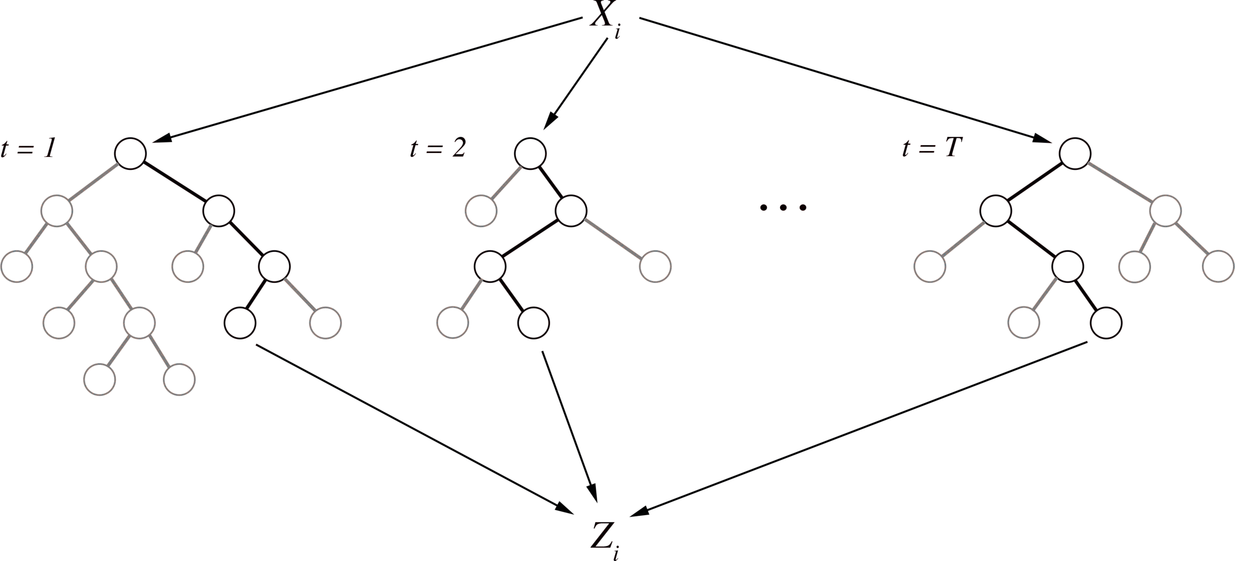
Generalized random intersection trees
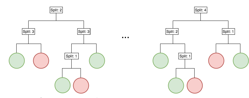
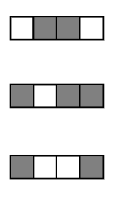
Encoding decision paths to extract active features
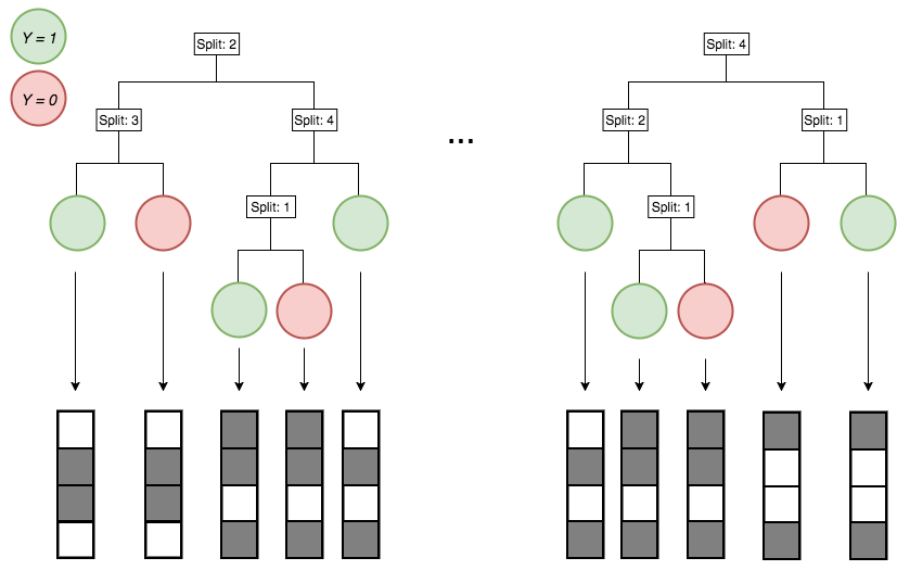
Active
Inactive
Continuous measurements
Binary features

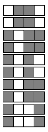
Encoding decision paths to extract enriched and depleted features
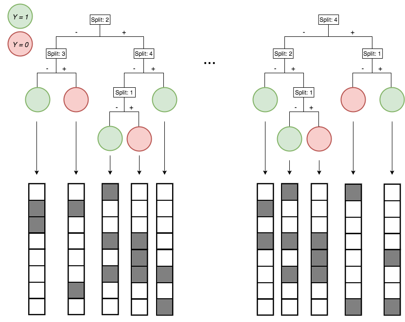
Enriched
Depleted
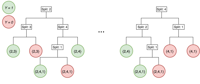
Generalized random intersection trees search for high-order interactions
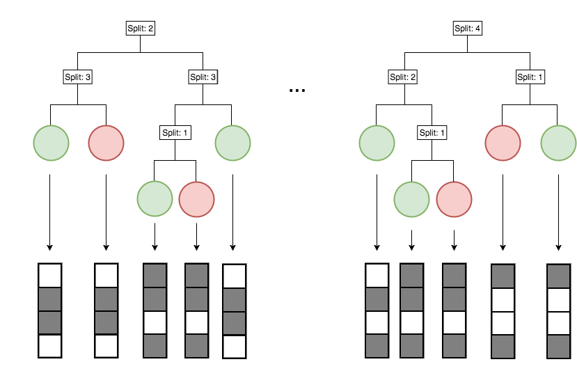
\cap
\cap
\cap
\cap
\{1,4\}
1. Iteratively re-weighted random forests
3. RIT on random forest decision paths
2. Decision path feature transformation
\mathbf{x}_1 \rightarrow \mathcal{I}_1 =
\mathbf{x}_n \rightarrow \mathcal{I}_n =
.
.
.
\emptyset
Encoding decision paths to extract prevalent decision rules
Continuous measurements
Binary feature encoding
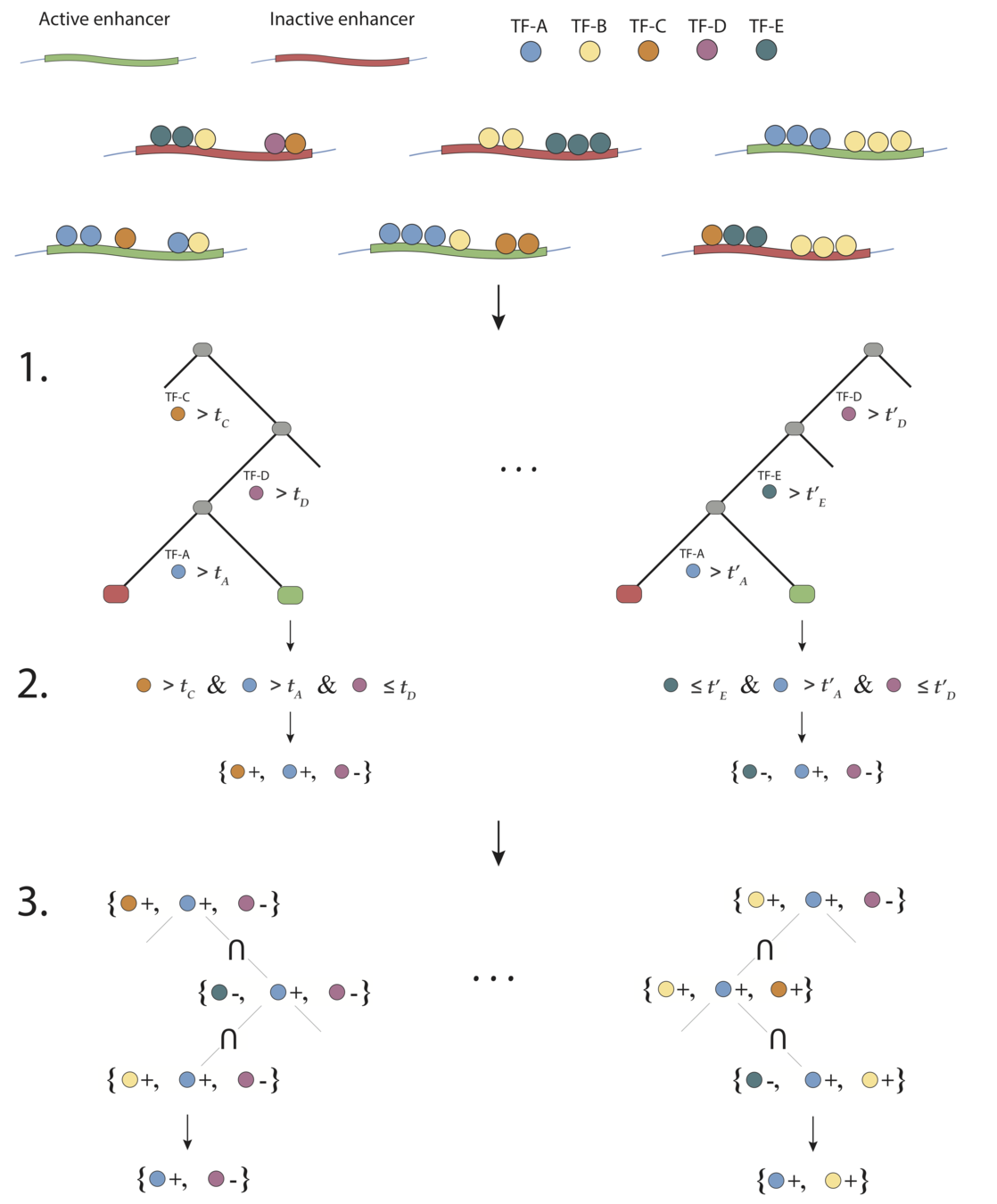
Decision rules
Encoding decision paths to extract prevalent decision rules
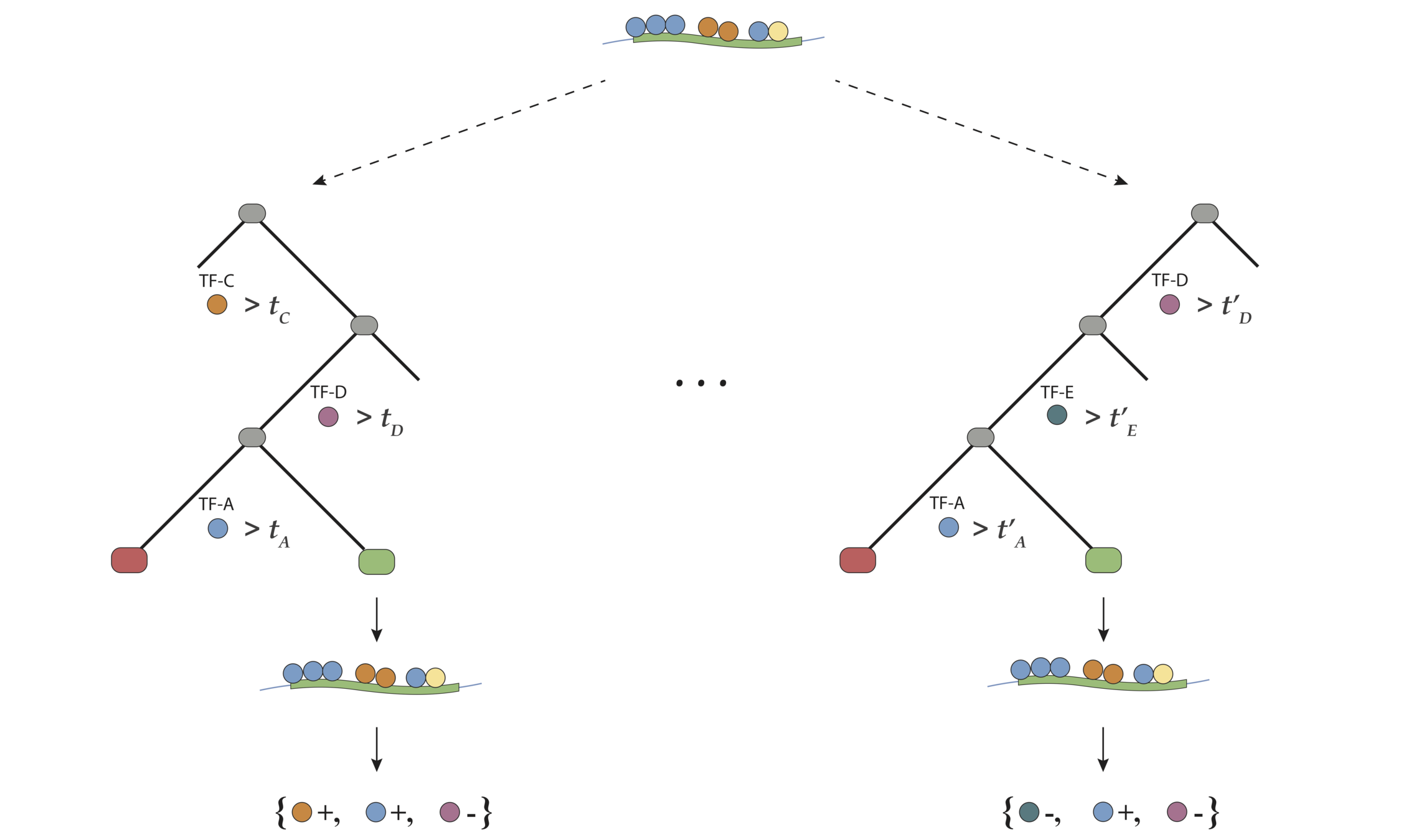
\mathbf{x}_i
S_{i_1}
S_{i_T}
. . .
Generalized random intersection trees search for high-order interactions

Prevalent interactions
Binary feature encoding
RIT
. . .
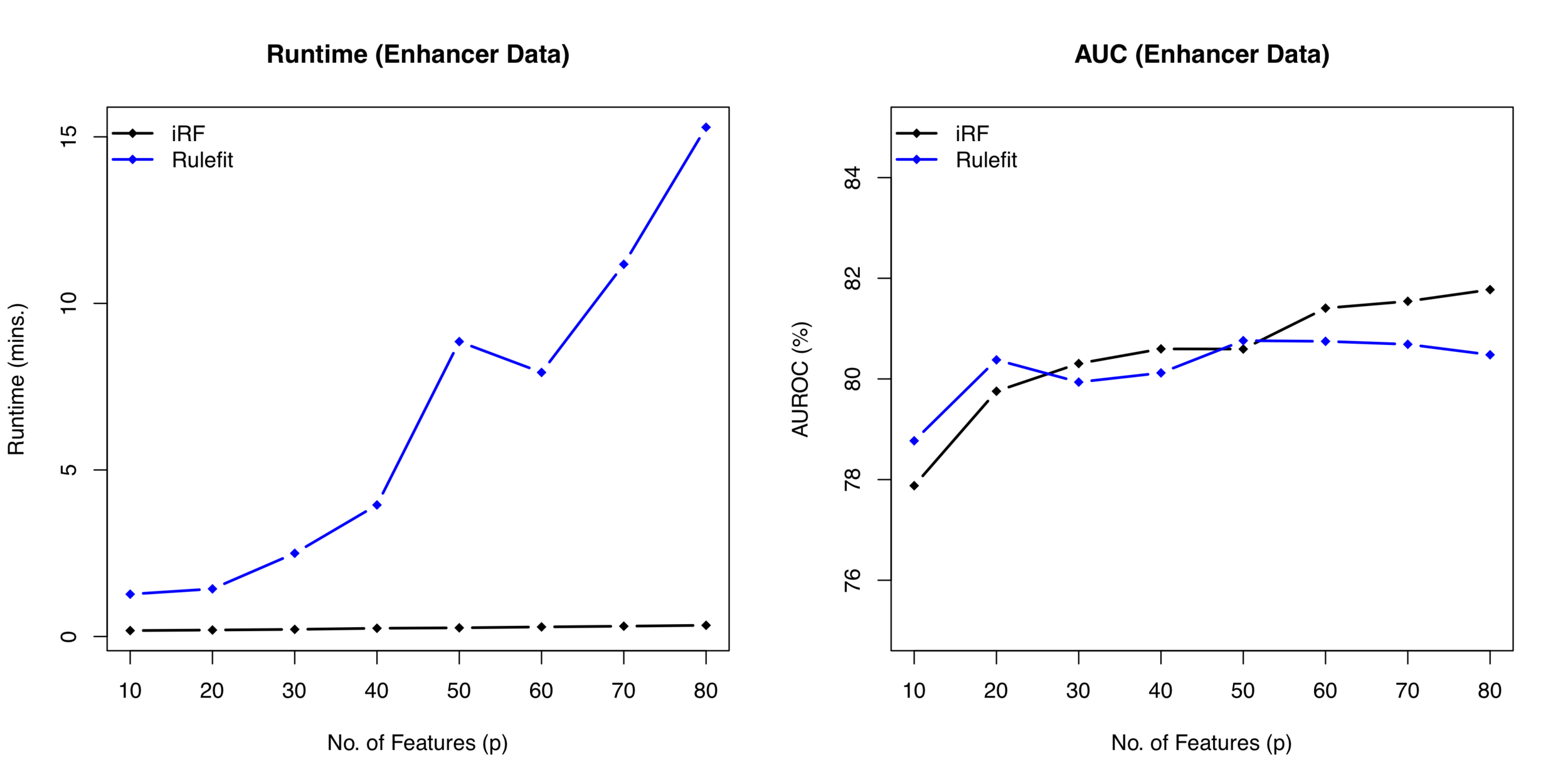
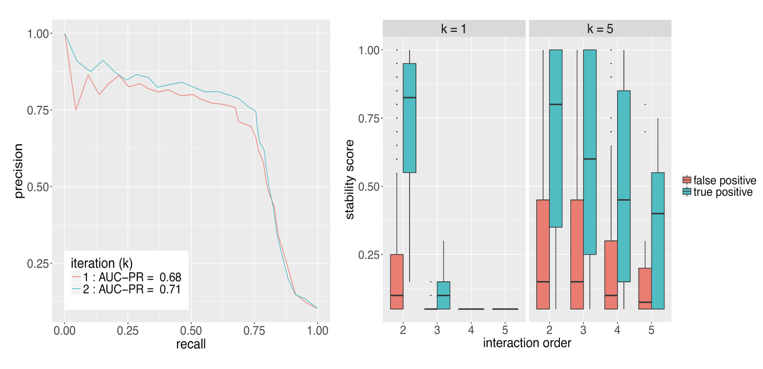
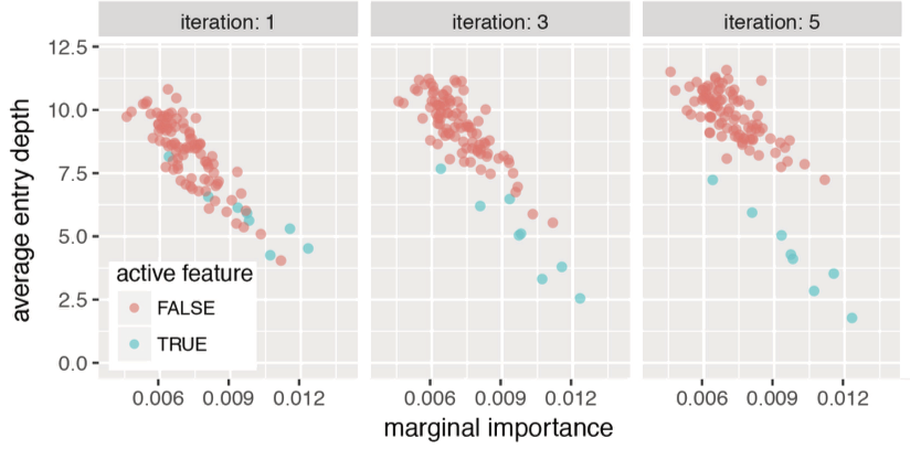
Runtime comparison between iRF and RuleFit
Evaluating interactions
PCS framework for veridical data science
("Veridical data science", Yu and Kumbier, 2020)
Predictability (from ML, Stats) evaluates whether models/results reflect external reality
Computability (from ML) enables domain-inspired simulations to compare against known structure
Stability (from Stats) assesses the reproducibility of results relative to data and model perturbations
The PCS framework unifies and expands on ideas from statistics and machine learning
Precision measures the predictive accuracy of an interaction across an RF
Precision:
P(y=1|S)=\frac{1}{T} \sum_{t=1}^T \frac{\sum_{i=1}^n I(S\subseteq \mathcal{I}_{i_t}) \cdot I(y_i = 1)}{\sum_{i=1}^n I(S\subseteq \mathcal{I}_{i_t})}
P(y=1|\{1, 4\}) = 4/6
P(y=1|\{1, 3, 4\}) = 3/4
Examples:
Prevalence measures the stability of an interaction across an RF
Prevalence:
P(S|y=1)=\frac{1}{T} \sum_{t=1}^T \frac{\sum_{i=1}^n I(S\subseteq \mathcal{I}_{i_t}) \cdot I(y_i = 1)}{\sum_{i=1}^n I(y_i = 1)}
P(\{1, 3, 4\}|y = 1) =3/5
P(\{1, 4\}|y = 1) =4/5
Examples:
Null metrics describe importance measures under simple structure computed from RF
Biology: TF enrichment among active enhancers
Null model: prevalence among inactive elements
Biology: cooperative binding among TFs
Null model: expected prevalence under independent selection
Biology: functional binding v. inactive binding
Null model: precision of interaction subsets
Bagging evaluates stability of interactions across entire iRF workflow relative to resampling
\cap
\cap
\cap
\cap
\cap
\cap
\cap
\cap
\{1,4\}
\{1,3\}
P(S|y=1)
P(S|y=1)
\dots
1. Iteratively re-weighted RF stabilize decision paths
2. gRIT searches for high-order interactions along decision paths
3. Importance metrics evaluate interactions in fitted RF
Outer layer bootstrap samples
\emptyset
\{1,4\}
Discovering "functional" TF binding and interactions in the Drosophila embryo
Joint work with Sumanta Basu, James B. Brown, Susan Celniker, Erwin Frise, and Bin Yu


Predicting enhancer activity throughout embryonic development
Enhancers: Pfeiffer et al. 2008, Fisher et al. 2012, Kvon et al. 2014
ChIP: MacArthur et al. 2009, Li et al. 2008, modENCODE/modERN consortia
x_1
x_2
\dots
y
iRF predicts stage-specific enhancer activity with high accuracy and recovers well-known pairwise interactions
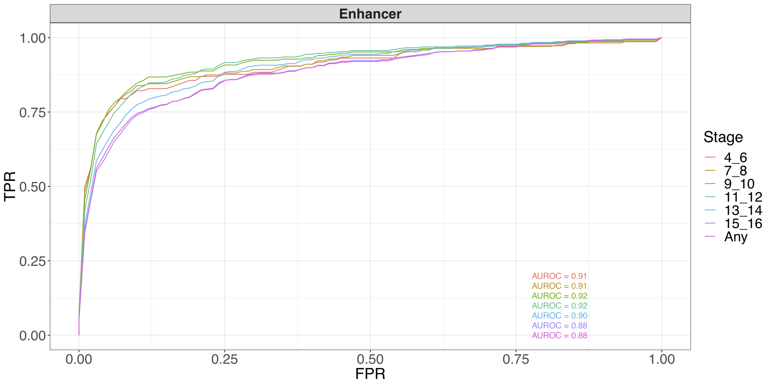
Early stage (not shown): 24 TFs; Basu, K., Brown, and Yu (2018)
All stages (shown): 307 TFs; K., Basu, Brown, Celniker, Frise and Yu
Predicting enhancer activity throughout embryonic development
Early stage (not shown): 24 TFs; Basu, K., Brown, and Yu (2018)
All stages (shown): 307 TFs; K., Basu, Brown, Celniker, Frise and Yu
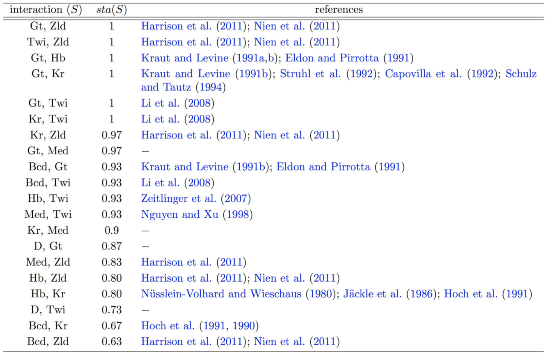
iterative Random Forests recover well-known pairwise interactions
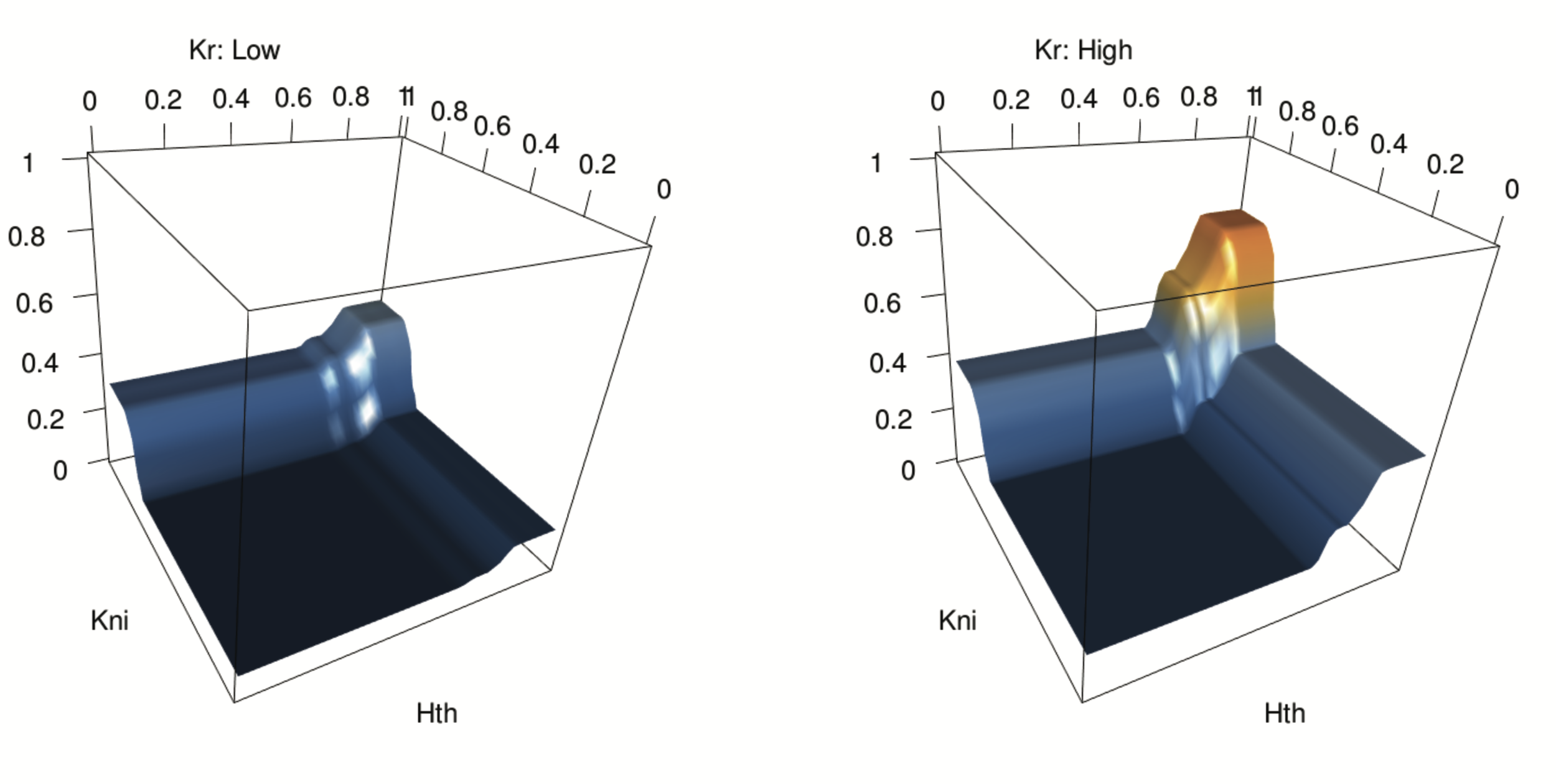
Novel order-3 interactions exhibit AND-like behavior (Hth, Kni, Kr)
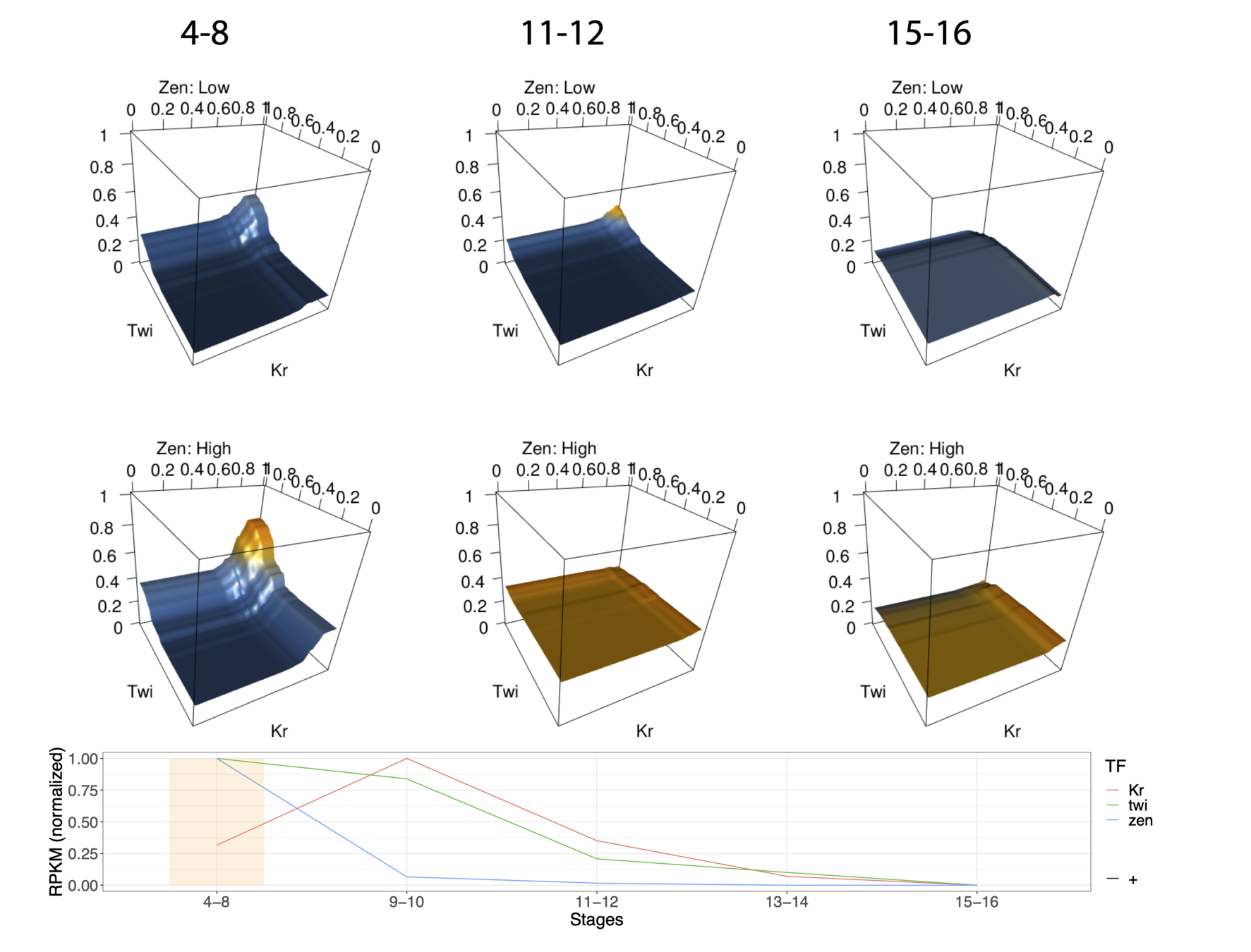
Novel interactions show strong concordance with temporal expression
siRF correctly identifies known regulators of eve
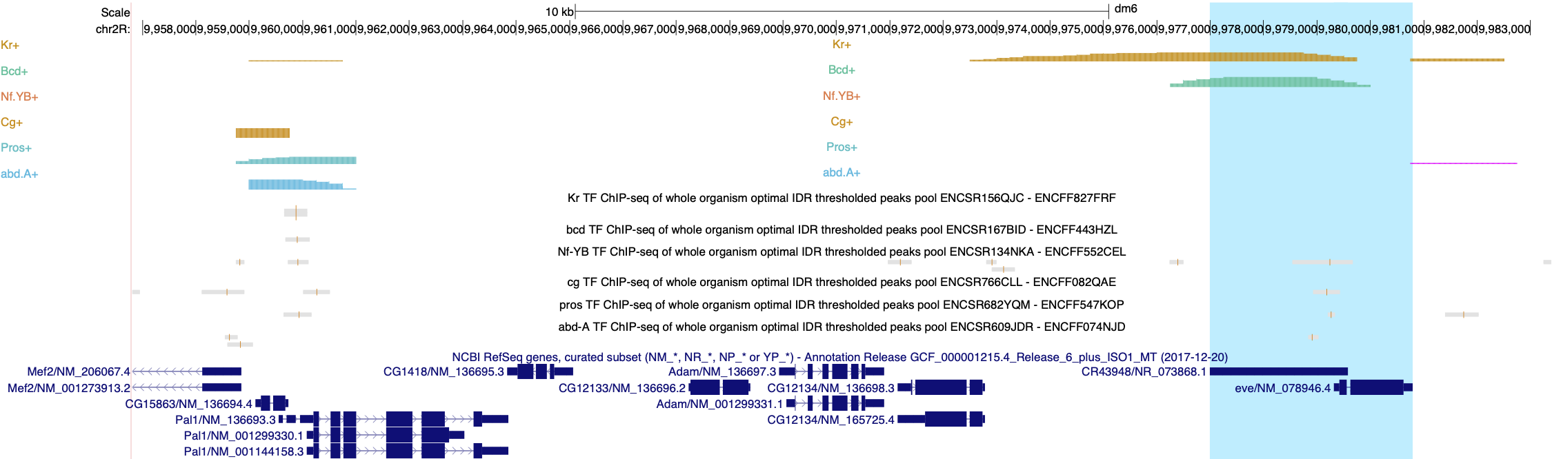
Binding of known regulators correctly identified by siRF and missed by IDR
Binding with no reported function identified by IDR and not called by siRF
siRF filters down to high-quality set of functional peaks
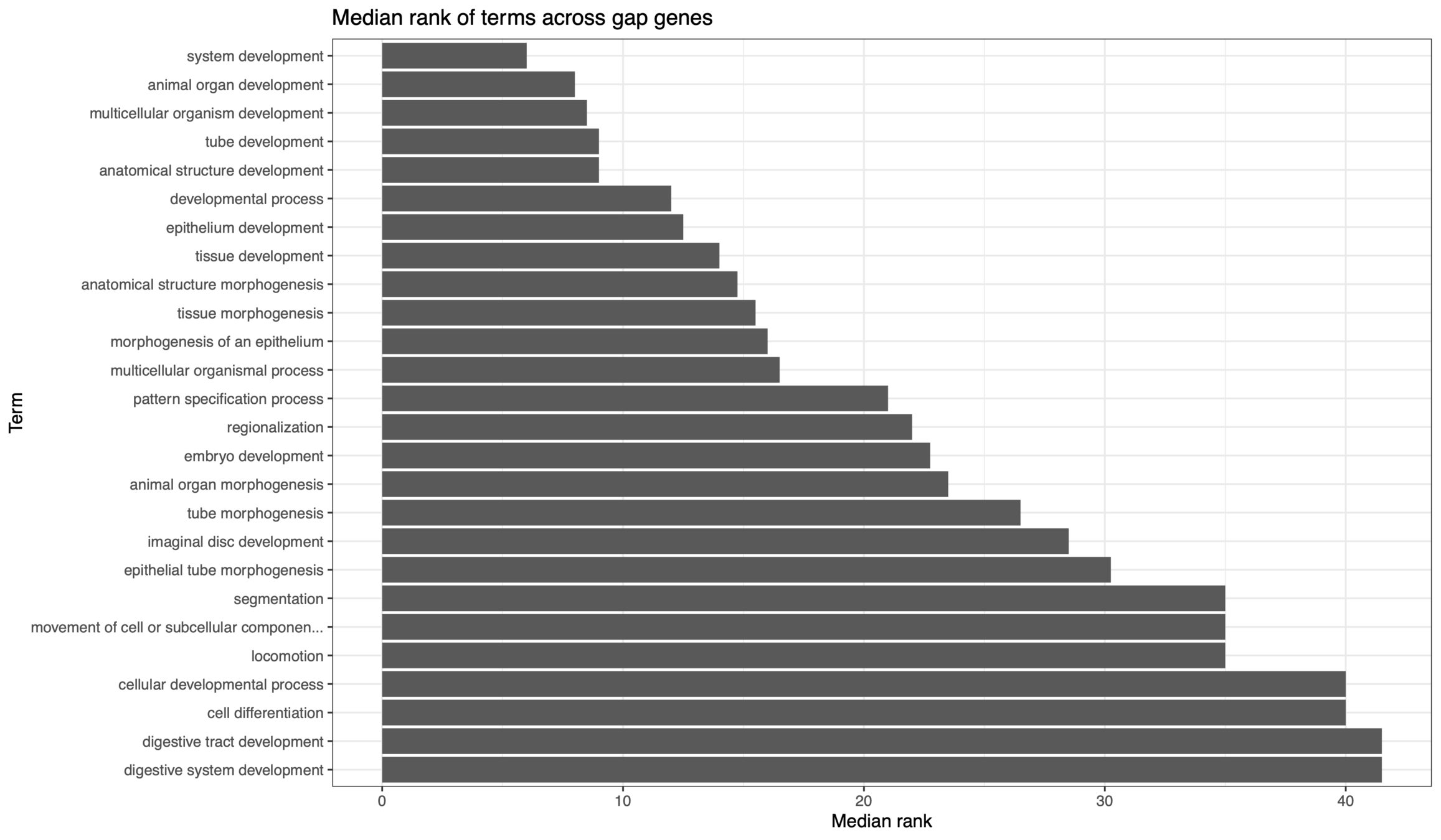
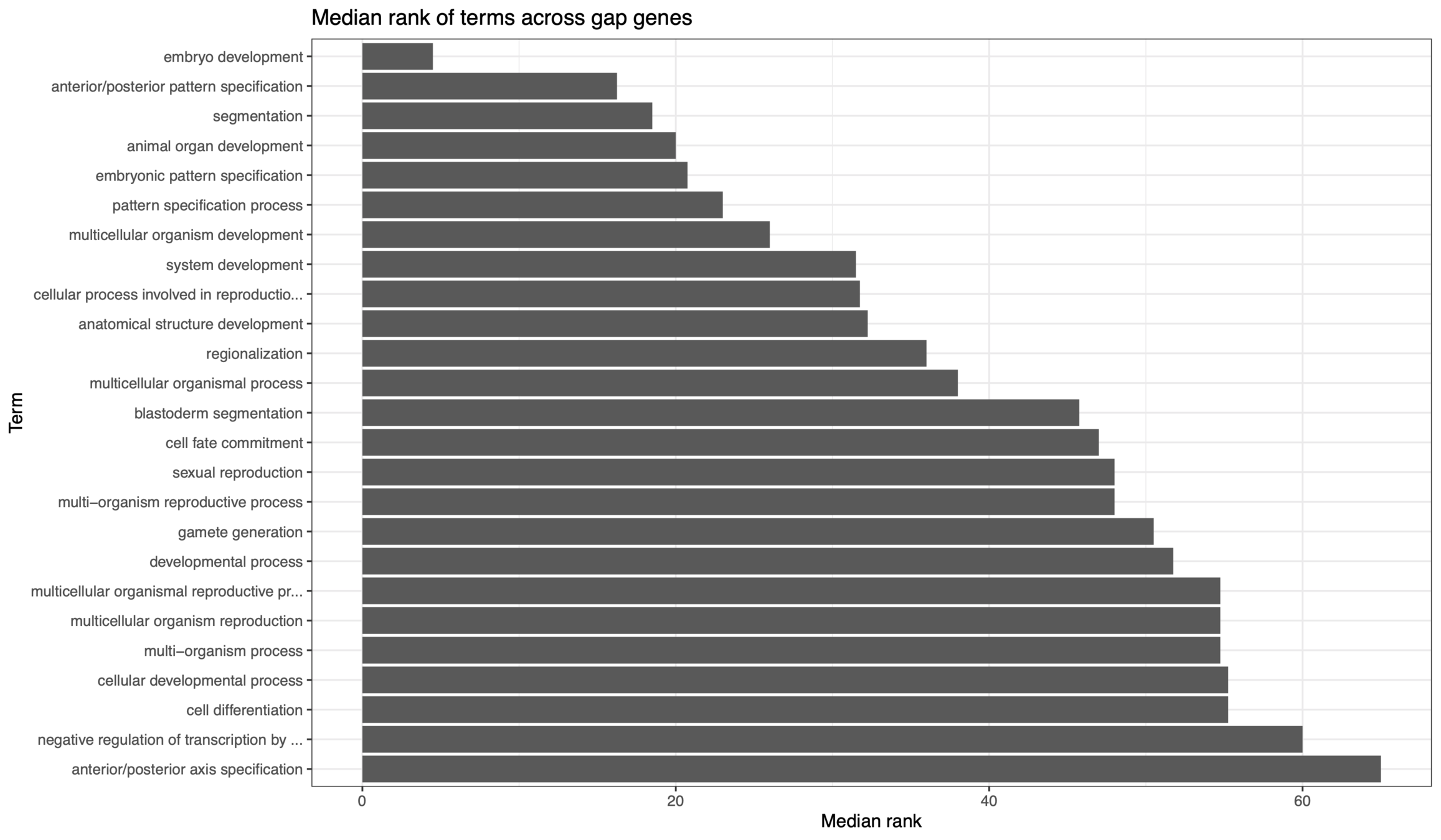
siRF functional binding GO term enrichment
IDR binding GO term enrichment
Figure: Wotton et al. (2015)
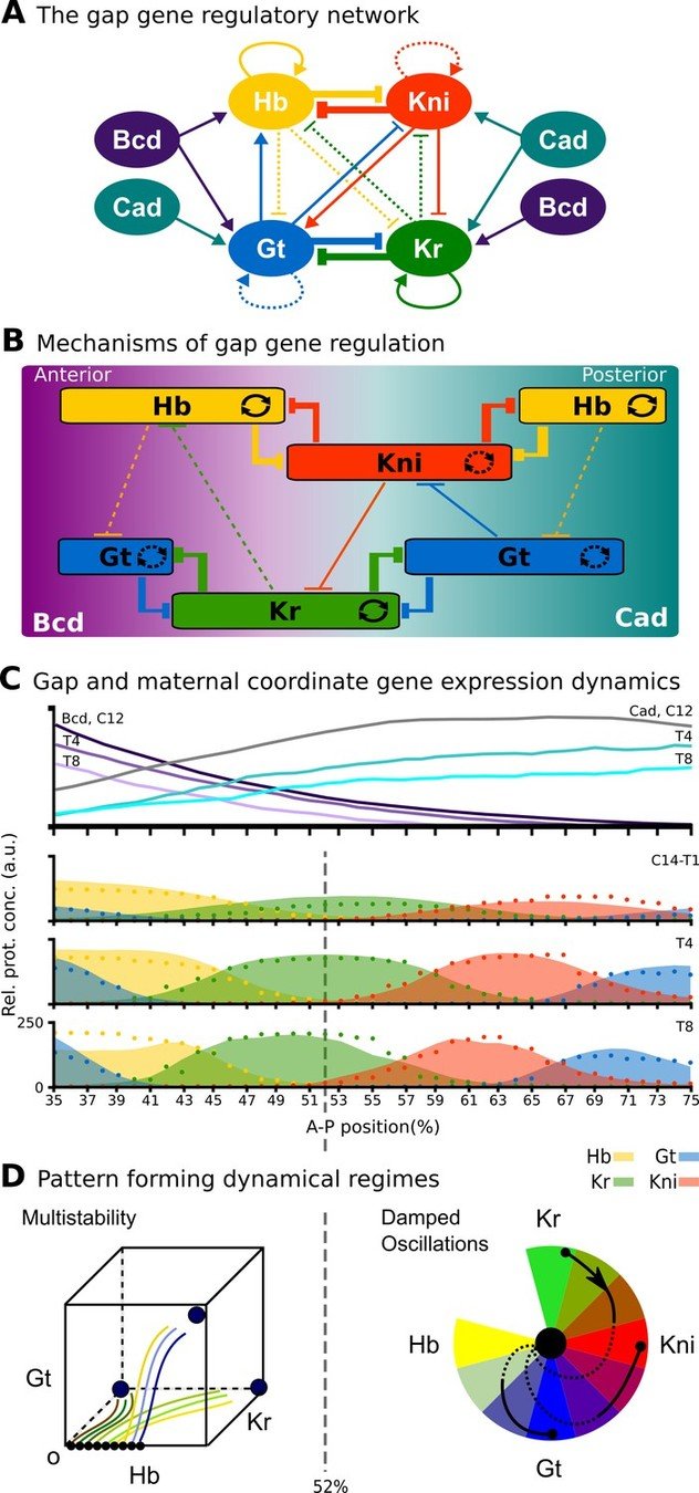
Gap gene network as validation
EpiTree pipeline for detecting epistatic interactions in the UK Biobank
Joint work with: Merle Behr, Aldo Cordova-Palomera, Matthew Aguirre, Euan Ashley, Atul J. Butte, Rima Arnaout, Ben Brown, James Priest, Bin Yu
New method EpiTree for epistasis discovery
- Flexible and non-linear mathematical form
- Suited to detect interactions of order > 2
- Entirely genetic
- Governed by epistasis (Morgan et al. 2018)
- Common trait
Positive control phenotype: red hair

- ~500,000 individuals
- Self-reported hair color
- 10,000,000 variants from array genotype data
UK Biobank
PCS inference for epistatic interactions
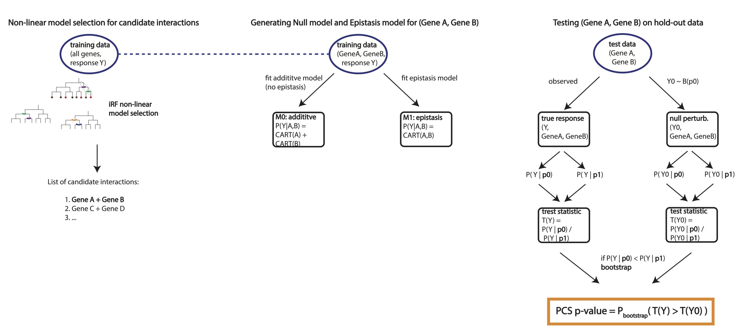
Learn models
Inference
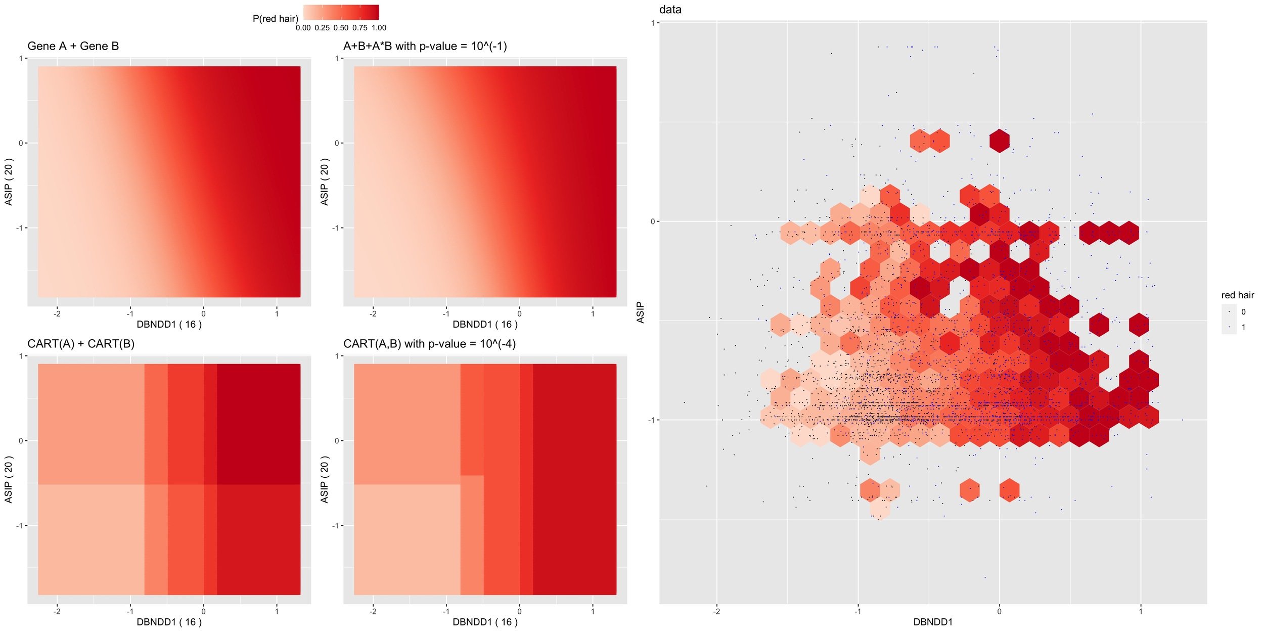
Predicting red hair in the UK biobank

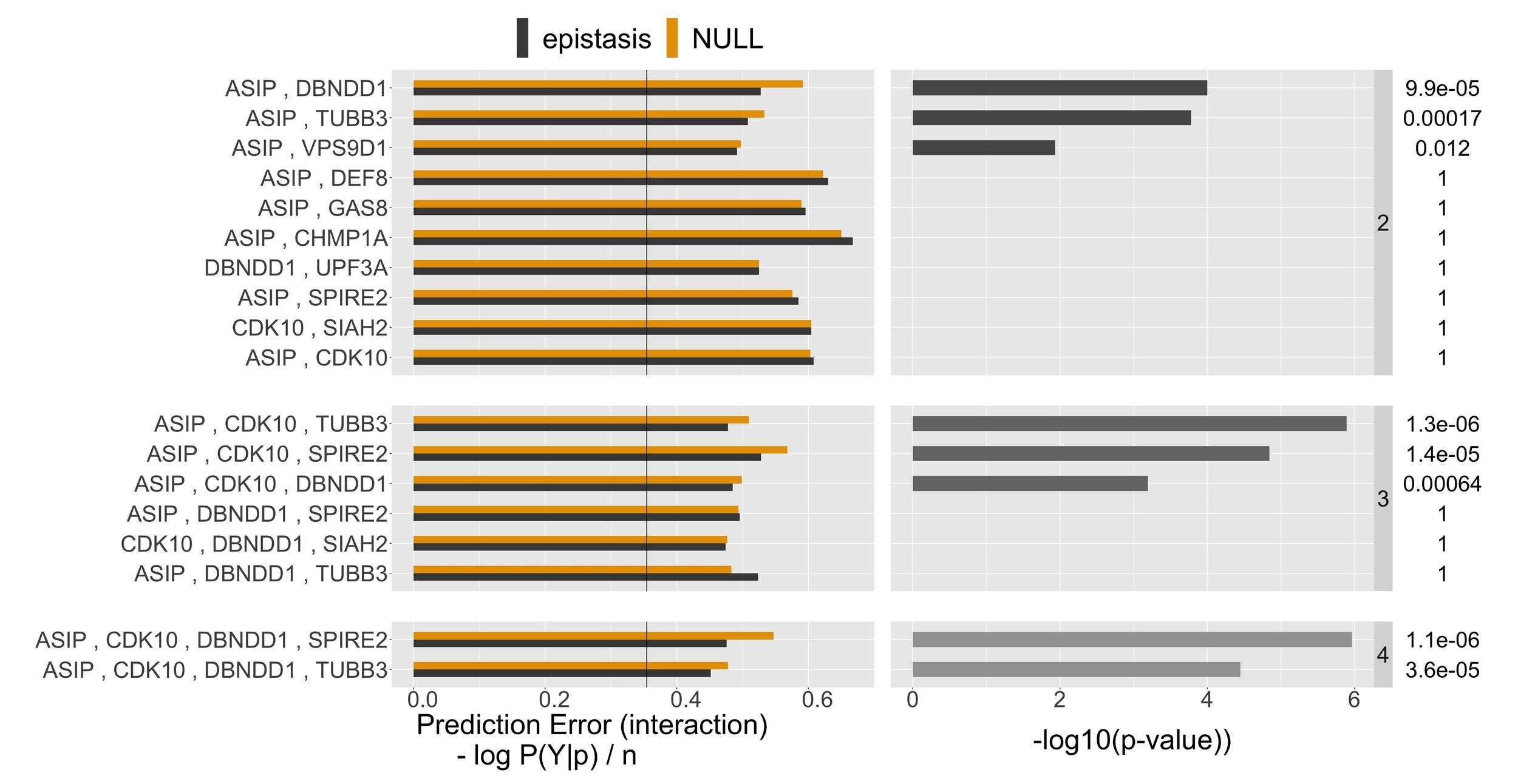
- Recovers known genetic determinants of hair color & pigmentation
- Interactions recapitulate results from Morgan et al. (2018)
- EpiTree does not require a priori knowledge of important/causal variants
siRF interactions capture non-linearities missed by multiplicative interactions
Next steps: capturing heterogeneity in ALS through localization
-
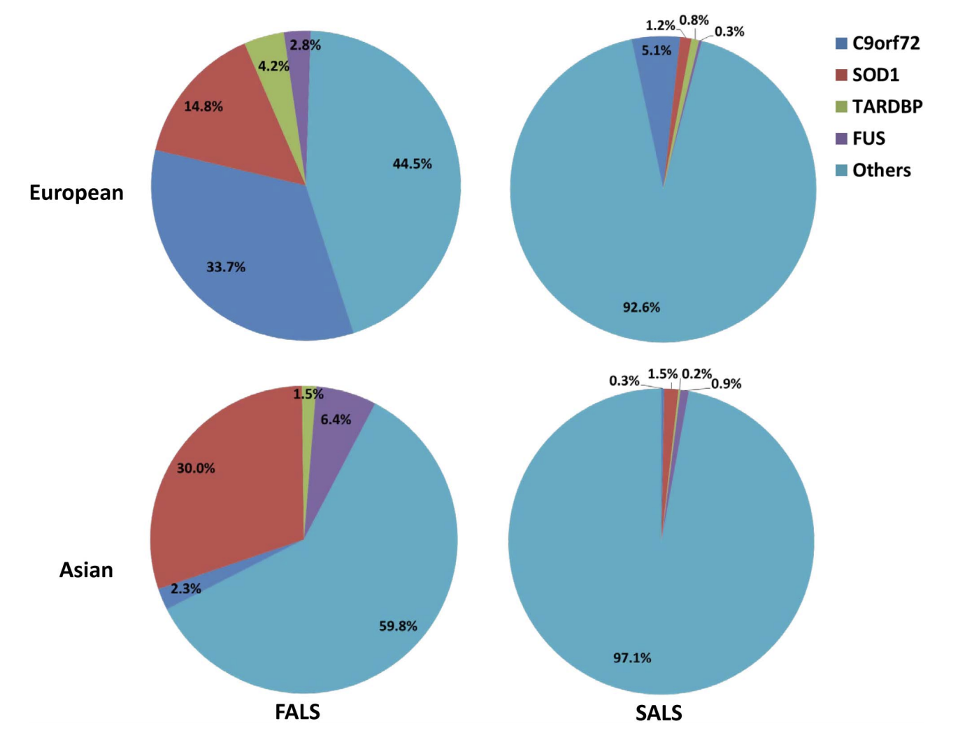
Amyotrophic lateral sclerosis (ALS) - fatal, neurodegenerative.
-
Over 25 known genetic causes. 90% of cases are sporadic (SALS); many of the familial (FALS) cases also have unknown cause
-
No effective treatments exist
Can we accelerate drug discovery by learning ALS subtypes and the patterns of dysregulation that define them?
Joint work with: Julia Lazzari-Dean, Maike Roth, Steven Altschuler, and Lani Wu
Figure: Zou, Z. Y. et al. (2017)
Summary
- iRF and siRF identify well known interactions in Drosophila and UK biobank data and posit new, high-order interactions.
- By decoupling interaction order from the computational cost of discovery, iRF and siRF allow us to investigate mechanisms in genome biology and beyond.
Ackowledgements


Drosophila
Sumata Basu, Erwin Frise, Susan Celniker, James B. Brown, Bin Yu


UK biobank
Merle Behr, Aldo Cordova-Palomera, Matthew Aguirre, Euan Ashley, Atul J. Butte, Rima Arnaout, Ben Brown, James Priest, Bin Yu
Thank You!
siRF - UCSF biostatistics
By kkumbier