SIESTA
post processing
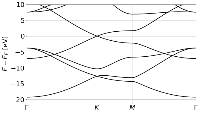
Band structure
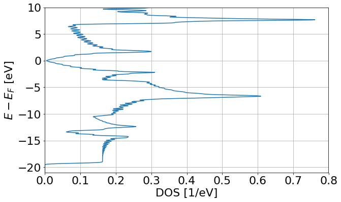
Density of States
Commandline tools
-
Mainly post processing based on a fix k-sampling
-
gnubands: generates plotable band structure file
from SIESTA's SYSTEM_LABEL.bands
-
Eig2DOS: generates plotable density of states file
from SIESTA's SYSTEM_LABEL.EIG
gnubands
jejbkv@c_cmcompsf17em-jejbkv:~/Al_bulk$ gnubands -h
 Usage: gnubands [options] [bandsfile|PIPE]

   bandsfile   : SystemLabel.bands
        PIPE   : < SystemLabel.bands

 Options:

     -h        : print help
     -G        : print GNUplot commands for correct labels to stderr
                 Suggested usage: prog options 2> bands.gplot 1> bands.dat
                    gnubands [options] 1> bands.dat 2> bands.gplot
                 and then:
                    gnuplot -persist bands.gplot
     -s arg    : only plot selected spin bands [1,nspin]
     -F        : shift energy to Fermi-level
     -b arg    : first band to write
     -B arg    : last band to write
     -e arg    : minimum energy to write
               :   If -F set, will be with respect
               :   to Fermi level
     -E arg    : maximum energy to write
               :   Note, see -e
     -o file   : specify output file (instead of piping)
               : if used with -G a file name file.gplot will be created
gnubands
jejbkv@c_cmcompsf17em-jejbkv:~/Al_bulk$ gnubands Al.bands
# GNUBANDS: Utility for SIESTA to transform bands output into Gnuplot format
#
#                                                  Emilio Artacho, Feb. 1999
#                                                   Alberto Garcia, May 2012
#                                           Nick Papior, April 2013, July 2016
# --------------------------------------------------------------------------
# E_F               =    -4.0678
# k_min, k_max      =     0.0000    3.3565
# E_min, E_max      =   -15.0494  174.4727
# Nbands, Nspin, Nk =     13     1  2101
# Using min_band, max_band =      1    13
# Total number of bands =     13
#
#        k            E
# --------------------------------------------------------------------------

      0.008601    -15.048400  1
      0.017203    -15.045500  1
      0.025804    -15.040600  1
      0.034406    -15.033900  1
      0.043007    -15.025100  1
      0.051609    -15.014400  1
      0.060210    -15.001800  1
      0.068812    -14.987100  1
      0.077413    -14.970500  1
                .
                .
                .
Eig2DOS
jejbkv@c_cmcompsf17em-jejbkv:~/Al_bulk$ Eig2DOS -h
 -------------------
 Usage: Eig2DOS [options] eigfile

        eigfile : SIESTA .EIG file

 OPTIONS:

 -h         Print this help
 -d         Print debugging info
 -e         Stop after printing Emin,Emax in file for selected bands
 -f         Shift energy axis so that Efermi is at 0
 -l         Use Lorentzian instead of Gaussian broadening
 -s arg     Broadening parameter in eV
 -n arg     Number of energy points at which to compute the DOS
 -m emin    Minimum energy in range
 -M emax    Maximum energy in range
 -b arg     Index of first band to consider
 -B arg     Index of last band to consider
 -k kfile   Use kfile for k-point weight information (.KP format)
 -------------------
Eig2DOS
jejbkv@c_cmcompsf17em-jejbkv:~/Al_bulk$ Eig2DOS Al.EIG
# EIG2DOS: Utility for SIESTA to obtain the electronic density of states
#  E. Artacho, Apr 1999, A. Garcia, Apr 2012
# ------------------------------------------
# Eigenvalues read from Al.EIG
# Using smearing parameter:   0.200
# Using    200 points in energy range
# Selected bands: 1 to: 13
# Emin, emax in file for selected band(s):    -14.9845100    143.2186600
# Nbands, Nspin, Nk   =     13     1   500
# E_F                 =    -4.0678 eV (NOT shifted)
# Broadening          =     0.2000 eV
#
#        E            N(up)  (=)   N(down)         Ntot
    -16.184510      0.000000      0.000000      0.000000
    -15.377459      0.000124      0.000124      0.000249
    -14.570408      0.040457      0.040457      0.080915
    -13.763357      0.077437      0.077437      0.154874
                                .
                                .
                                .
                                .
                                .
sisl : a python based tool
CDF.Save true
CDF.Compress 9
SaveHS true
SaveRho true
sisl : a python based tool
nkx,nky,nkz = 10,10,1                              # number of kpoints in each direction
E = np.linspace(Emin, Emax, 500)                   # Energy range
bz = MonkhorstPack(H, [nkx, nky, nkz]).asaverage() # Brilloun-zone sampling
dos_data = bz.DOS(E)                               # The actual calculation of the DOS

plot(E,dos_data)                                   # plot it with matplotlib like this
fdf = get_sile('RUN.fdf') # Identify calculation based on the fdf file
H = fdf.read_hamiltonian() # Read in Hamiltonian, this will trow an error
# if the Hamiltonian was not calculated!calculate DOS
Read in SIESTA output
bz = BandStructure(H, [[0,0,0], [2./3, 1./3, 0], [0.5, 0.5, 0], [1,1,1]], # BZ path
                       400,                                               # number ok kpoints
                   name=[r'$\Gamma$', r'$K$', r'$M$', r'$\Gamma$'])       # named k-points
linear_k, k_tick, k_label = bz.lineark(True) # get tick position and tick labels
bands = bz.eigh()      # the actual calculation of the band structure
plt.plot(linear_k,bands); # plot like this
# puting labels
plt.ylabel(r'$E-E_F$ [eV]')
plt.xlim(linear_k[0], linear_k[-1]);
plt.xticks(k_tick, k_label);
calculate bands
SIESTApost processing
By László Oroszlány


