How Not to Write a High-Performance N-body Code
Lehman Garrison (SCC, formerly CCA)
FWAM, High-Performance Computing Case Study
Oct. 28, 2022

https://github.com/lemmingapex/N-bodyGravitySimulation
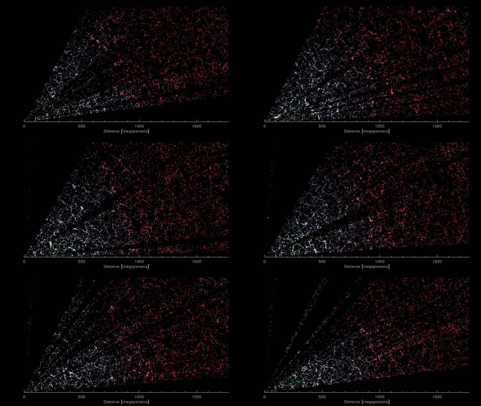
The Large-Scale Structure of the Universe

First 8 weeks of DESI Survey data (2021; Credit: D. Schlegel/Berkeley Lab)
Telescope surveys see that galaxies cluster together, forming a "cosmic web"
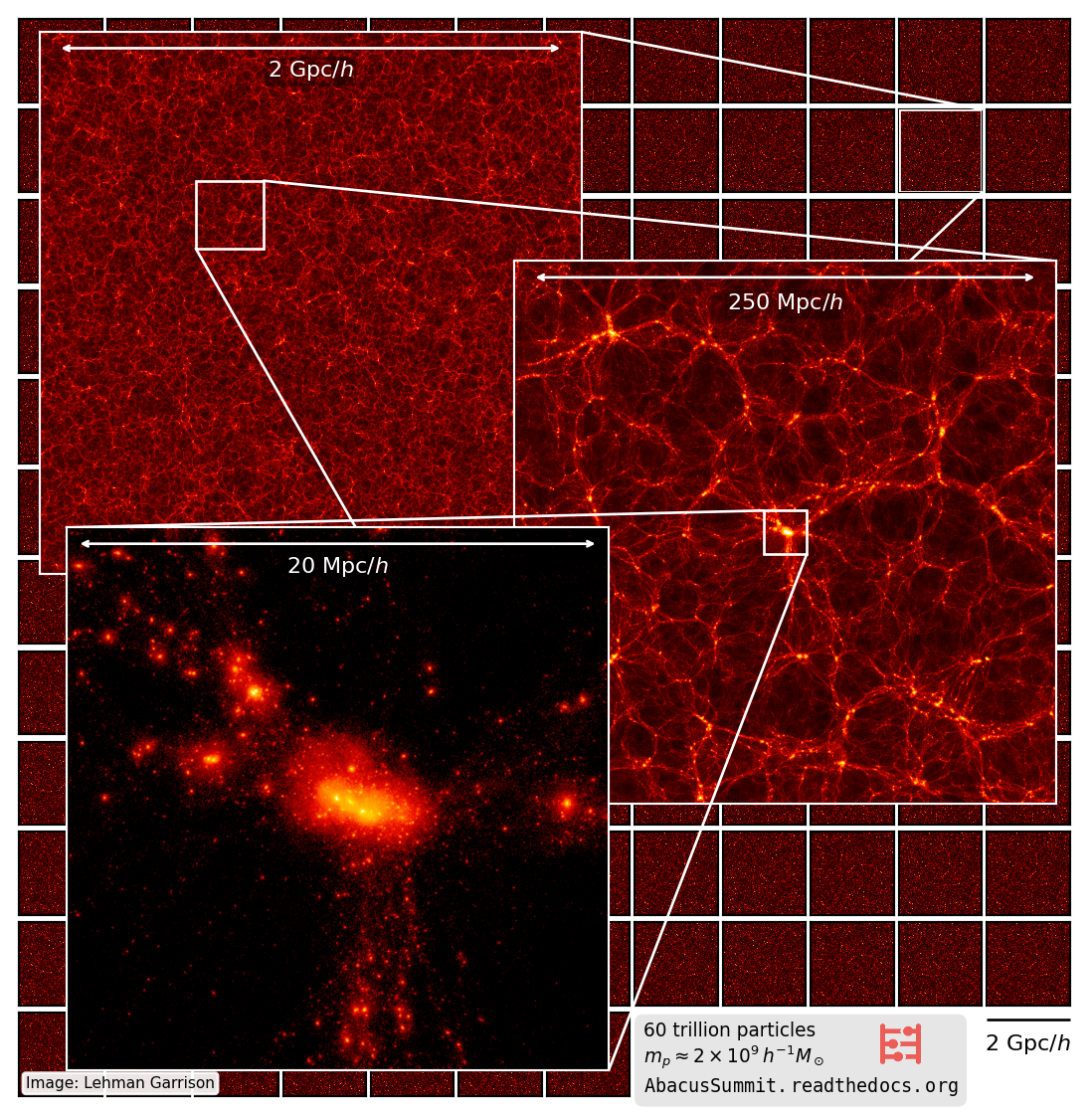
Simulating the Cosmic Web
- Gravitational instability in an expanding universe explains the cosmic web
- Can simulate by treating all matter as collisionless particles
- Ignore gas dynamics; good enough for large scales
- Discretize the matter into N particles, evolve equations of motion under Newtonian gravity in a GR background
Credit: Benedikt Diemer & Phil Mansfield
N-body: the computational task
- Integrate equations of motion of each particle using leapfrog
- Requires gravitational force at each time step: $$ \vec{F_i} \propto \sum_j^N \frac{\vec{r_j} - \vec{r_i}}{|\vec{r_j} - \vec{r_i}|^3} $$
- Naive time complexity \( \mathcal{O}(N^2) \)
- Must also respect periodic boundary conditions
- Won't use \( \mathcal{O}(N^2) \) on large scales; might still on small scales
It gets worse...
- Tiny galaxies shine across vast cosmic distances
- Need high mass resolution, large simulation volume
- Non-trivial gravitational coupling of large scales to small
- Typical flagship N-body simulations have 1+ trillion particles in 2022
- 1 trillion particles
- Typically 32+ TB of particle state
- All-to-all communication
- Thousands of time steps
- Tightly coupled

The Abacus N-body Code
- New code for cosmological N-body simulations (Garrison et al., 2021)
- Based on new multipole method with exact near-field/far-field split
- Near field GPU-accelerated; far field CPU SIMD-accelerated
- Fastest published per-node performance of any cosmological N-body code
- Tiny force errors, typically \(10^{-5}\) (frac.)
- Written in C++/CUDA, with MPI+OpenMP parallelization


Hearken back to 2013...
- GPU computing was just entering mainstream
- Beyoncé only had 17 Grammys
- Few academic GPU clusters
- A single node could house enough GPUs to run a simulation, but how do you hold it in memory? With disk!
- Abacus "slab pipeline" designed to only need a thin slice of the simulation in memory
- Rest of the simulation can be on disk (2013), on another node (2020), etc
- Lots of IO optimization

Abacus cluster in the Harvard Astro Dept. basement


Lesson #0: Don't cook your hard drives
Abacus Slab Pipeline
Slab 7
Slab 6
Slab 5
Slab 4
Slab 3
Slab 2
Slab 1
\(X\)-axis
Abacus Slab Pipeline
Slab 7
Slab 6
Slab 5
Slab 4
Slab 3
Slab 2
Slab 1
Read
Abacus Slab Pipeline
Slab 7
Slab 6
Slab 5
Slab 4
Slab 3
Slab 2
Slab 1
Read
Far-field
force
Abacus Slab Pipeline
Slab 7
Slab 6
Slab 5
Slab 4
Slab 3
Slab 2
Slab 1
Read
Far-field
force
Abacus Slab Pipeline
Slab 7
Slab 6
Slab 5
Slab 4
Slab 3
Slab 2
Slab 1
Read
Near-field
force (GPU)
Abacus Slab Pipeline
Slab 7
Slab 6
Slab 5
Slab 4
Slab 3
Slab 2
Slab 1
Read
Near-field
force (GPU)
Far-field
force
Kick/Drift/
Multipoles
Abacus Slab Pipeline
Slab 7
Slab 6
Slab 5
Slab 4
Slab 3
Slab 2
Slab 1
Read
Near-field
force (GPU)
Far-field
force
Kick/Drift/
Multipoles
Write
Abacus Slab Pipeline
Slab 7
Slab 6
Slab 5
Slab 4
Slab 3
Slab 2
Slab 1
Read
Near-field
force (GPU)
Far-field
force
Kick/Drift/
Multipoles
Write
Abacus Slab Pipeline
- Uses the exact decomposition of the multipole method to process the simulation volume slab-by-slab
- FFT convolution of multipoles happens after pipeline, produces far-field for next step
- Pipeline actually expressed as an event loop (code example)
- Easily incorporates asynchronous activity, like IO, GPU, or MPI
void slab_pipeline(){
  while(!Finish.doneall()){
      if(LaunchRead.precondition()) LaunchRead.action();
      if(NearForce.precondition())  NearForce.action();
      if(FarForce.precondition())   FarForce.action();
      if(Kick.precondition())       Kick.action();
      if(Drift.precondition())      Drift.action();
      if(Finish.precondition())     Finish.action();
  }
}

class NearForce : Stage {
    int precondition(int slab){
        for(int i = -RADIUS; i <= RADIUS; i++){
            if(!Read.done(slab+i)) return 0;
        }
        return 1;
    }
    void action(int slab){
        SubmitToGPU(slab);
    }
};
From single-node to multi-node
- From a node's perspective, it doesn't matter if the not-in-memory particles are on disk or on another node
- In 2018, we added MPI parallelization, reusing the slab decomposition
- This 1D parallelization had perfect scaling to 140+ nodes on Summit
- Any larger and the domains become too thin for halo finding
- Rolling decomposition: a node ends with a different domain than it starts with
- No boundary approximations!

Custom OpenMP Scheduler
- Modern systems have "Non-Uniform Memory Access" (NUMA)
- Cores access memory on the same socket (NUMA node) faster
- Abacus slabs are divided over sockets. Want the CPUs to only work on rows on that socket.
-
Abacus used to use static scheduling, but started choking on load balancing in big sims
Socket 1
Socket 2
CPU 1
CPU 1
CPU 2
CPU 3
CPU 3
CPU 4
void KickSlab(int slab){
    #pragma omp parallel for schedule(???)
    for(int j = 0; j < nrow; j++){
        KickRow(slab,j);
    }
}
CPU 2
CPU 4
Custom OpenMP Scheduler
- OpenMP 4 doesn't have a "dynamic-within-socket" schedule
- Nor does it let you write a custom scheduler
- But we can hack one together...
- Use OpenMP tasks
- Atomic addition to grab next loop iteration
- 25% improvement in performance of far-field calculation
- But can't use "reduction" clauses, have to implement manually...
#define NUMA_FOR(N)
    _next_iter[0] = 0;   // node 0
    _last_iter[0] = N/2;

    _next_iter[1] = N/2; // node 1
    _last_iter[1] = N;

    #pragma parallel
    for(int j; ; ){
        #pragma atomic capture
        j = _next_iter[NUMA_NODE]++;
        if(j >= _next_iter[NUMA_NODE+1])
            break;
#pragma omp parallel for
for(int j = 0; j < nrows; j++){
    KickRow(slab,j);
}
NUMA_FOR(nrow)
    KickRow(slab,j);
}
Given the following code:
Rewrite as:
Lesson #1: don't let your threads access memory on the wrong NUMA node
Lesson #1b: Don't write a custom OpenMP scheduler
Lesson #1a: don't let your threads access memory on the wrong NUMA node
Loop Unrolling & SIMD Metacode
void multipoles(const double *pos, const int N, double *multipole){
    for(int i = 0; i < N; i++){
        double mx = 1.;
        for(int a = 0; a <= ORDER; a++){
            double mxy = mx;
            for(int b = 0; b <= ORDER - a; b++){
                double mxyz = mxy;
                for(int c = 0; c <= ORDER - a - b; c++){
                    multipole[a,b,c] += mxyz;
                    mxyz *= pos[2,i];
                }
                mxy *= pos[1,i];
            }
            mx *= pos[0,i];
        }
      }
   }
}
Performance: \(7\times10^6\) particles/sec (1 core)
print('double mx = 1.;')
for a in range(ORDER + 1):
    print('double mxy = mx;')
    for b in range(ORDER - a + 1):
        print('double mxyz = mxy;')
        for c in range(ORDER - a - b + 1):
            print(f'multipoles[{a},{b},{c}] += mxyz;')
            print('mxyz *= pos[2,i];')
        print('mxy *= pos[1,i];')
    print('mx *= pos[0,i];')
\(19\times10^6\) particles/sec
print('__m512d mx = _mm512_set1_pd(1.);')
for a in range(ORDER + 1):
    print('__m512d mxy = mx;')
    for b in range(ORDER - a + 1):
        print('__m512d mxyz = mxy;')
        for c in range(ORDER - a - b + 1):
            print(f'multipoles[{a},{b},{c}] = '\
              f'_mm512_add_pd(multipoles[{a},{b},{c}],mxyz);')
            print('mxyz = _mm512_mul_pd(mxyz,pos[2,i]);')
        print('mxy = _mm512_mul_pd(mxy,pos[1,i]);')
    print('mx = _mm512_mul_pd(mx,pos[0,i]);')
\(54\times10^6\) particles/sec
Loop Unrolling & SIMD Metacode
Lesson #2: don't trust the compiler to optimize complicated, performance-critical loops!

Other tricks: interleaving vectors, FMA, remainder iterations
PTimer Cache Line Contention
- Abacus PTimer (“parallel timer”) is used to profile performance-intensive, multi-threaded loops
- Each thread has a binary flag that it sets when it is active
- All flags were in a contiguous array
- 20 threads fighting for the same two cache lines inside tight nested loops
- Resolving this gave an immediate 50% CPU performance boost
-
Typical cache line size 64 bytes
-
Keep threads away from each other by at least this much
-

Lesson #3: don't share cache lines, especially in tight loops
GPU Data Model: Cells vs. Pencils
- Old version of GPU code processed cell pairs
- NVIDIA A100 GPU: 1500 GB/s memory bandwidth
- 125 Gparticles/sec
- 20 TFLOPS compute
- 770 Gforces/sec
- 770/125 = 6 forces per load
- Each particle should be used at least 6 times per load to shared mem
- 25 GB/s host to device PCIe bandwidth
- 2 Gparticles/sec
- 770/2 = 385 forces per host-device transfer
- Pencil-on-pencil
- Each particle acts on 5 sink pencils, 5 cells each
- Need at least 15 particle per cell—not bad!

Lesson #4: don't send data to the GPU unless you have a lot of floating-point work to do on it
What did we do with all this?

- 60 trillion particles
- More particles than all N-body simulations ever run, combined
- Performance of 300+ trillion directs/sec
- 7+ PB of raw outputs, processed and compressed to 2 PB
- 60% of theoretical peak usage of Summit GPUs
- Primary N-body simulation suite used by the DESI galaxy survey (Stage-IV DOE Dark Energy Experiment)
- Public data release: abacusnbody.org
Conclusions
- Many lessons about HPC learned from mistakes made in the Abacus code
- Don't cook hard drives
- Don't use static scheduling as a replacement for NUMA-awareness
- Don't trust compiler unrolling of complicated loops
- Don't let threads work within the same cache line
- Don't send data to the GPU unless you have lots of work to do on it
- Event loops are a powerful simulation programming model
- If you have a better approach for one of these problems, I'm eager to talk about it!
- Many other optimizations I didn't get to talk about:
- Thread pinning
- Memory allocators (tcmalloc)
- GPU memory pinning
- Ramdisk/mmap
- MPI point-to-point vs all-to-all

-
Checksumming
-
Compression/file formats
-
Representation of particle positions
-
SSD TRIM
-
GPU intermediate accumulators
Abacus FWAM Presentation
By Lehman Garrison
Abacus FWAM Presentation
- 334


