Gaussian Graphical Models in Multiple Omics Data Analysis: Theory and Applications with GmGM
Luisa Cutillo, l.cutillo@leeds.ac.uk, University of Leeds
in collaboration with
Andrew Bailey, and David Westhead, UoL
Sections
- Background on Gaussian Graphical models
- Our Approach:
GmGM

- Practical tutorial in github codespaces

Background on Gaussian Graphical Models (GGM)

Part 1
What is a GGM?
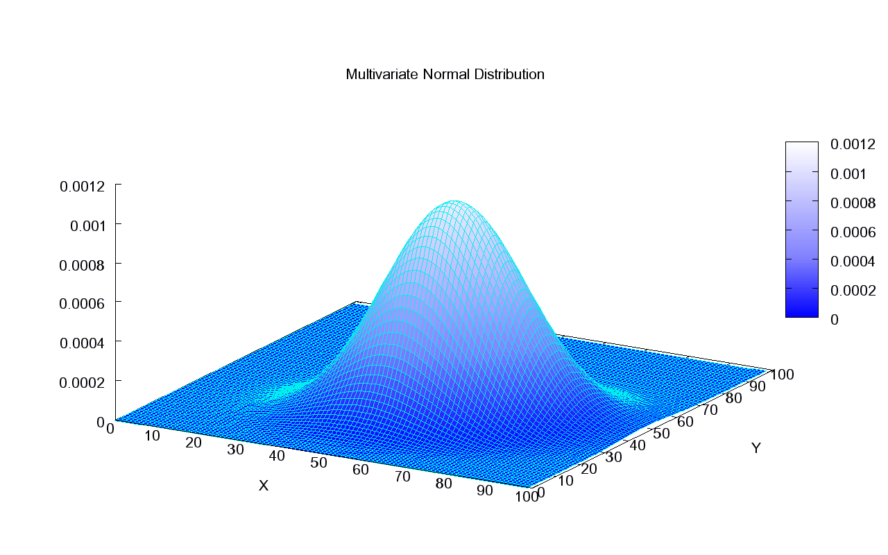
It is just a multivariate Gaussian distribution in !
Precision matrix


p= number of features,
What makes this a Graphical model?
We need to define a graph G(V,E) !

Set of Vertexes V=
Set of Edges E = Precision matrix
Markov Property:
Nodes 1 and 5 are conditionally independent given node 2
Edges correspond to direct interactions between nodes
Partial correlations via
partial correlation
Conditional Independence = SPARSITY!
A hypothetical example of a GGM on psychological variables. (Epskamp at all 2018)
Fatigue
Insomnia
Concentration
(Dempster, 72) it encodes the conditional independence structure
Focus on
Expresses the dependency graph
Example: Random Walk
What is the precision matrix?
About Sparsity...
- We want to study GGMs where is sparse
- This means more conditional independent variables
- Fewer elements to estimate -> Fewer data needed
Sparsity assumption => max graph degree d<<p
is reasonable in many contexts!
Example: Gene interaction networks
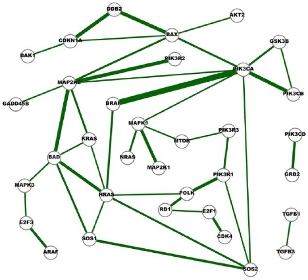
Example: Genes Interaction Networks Inference
- Inference 15 cancer networks and 10 normal networks using The Cancer Genome Atlas (TCGA) RNA-Seq gene expression data and GGM
- Subsets of genes outlined in the KEGG cancer pathways
- Networks were compared to further identify cross-cancer gene interactions.
Fig. 6. A network of strong cross-cancer interactions. Cancer Genetic Network Inference Using Gaussian Graphical Models. (2019) Zhao and Duan.
About Sparsity...
However the " Bet on Sparsity principle" introduced Tibshirani 2001, "In praise of sparsity and convexity":
(...no procedure does well in dense problems!)
- How to ensure sparsity?
Graphical Lasso (Friedman, Hastie, Tibshirani 2008):
imposes an penalty for the estimation of
Limitation
- Assumption of independence between features and samples
- Finds graph only between features
Features
Samples
Data
Main Aim:
Remove the independence assumption
Graph estimation without independence assumption

- Feature independence or data point independence is a model choice issue.
- General framework that models conditional independence relationships between features and data points together.
Deal with estimating a sparse graph that interrelates both features and data points .
-
video data example (Kalaitzis et al., 2013): both the frames (pictures over time) and the image variables (pixels) are correlated.

-
Single cell data: extract the conditional independence structure between genes and cells, inferring a network both at genes level and at cells level.
Cells
Genes
| 2 | ... | 10 |
|---|---|---|
| : | ... | : |
| 5 | ... | 7 |
Graph estimation without independence assumption
Bigraphical lasso: A different point of view
Preserves the matrix structure by using a Kronecker sum (KS) for the precision matrixes
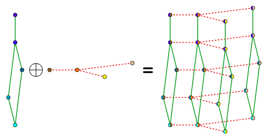

KS => Cartesian product of graphs' adjacency matrix
(eg. Frames x Pixels)

Bigraphical lasso: A different point of view
(kalaitzis et al. (2013))
Limitations:


- Space complexity: There are dependencies but actually implemented to store elements
- Computational time: Very slow, could only handle tens of samples.
We exploit eigenvalue decompositions of the Cartesian product graph to present a more efficient version of the algorithm which reduces memory requirements from O(n^2p^2) to O(n^2+ p^2).
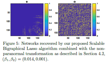
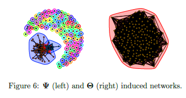
mEST dataset: 182 mouse embryonic stem cells (mESCs) with known cell-cycle phase. We selected a subset of 167 genes involved in the mitotic nuclear division (M phase) as annotated in DAVID database. Buettner et al. (2015)
https://github.com/luisacutillo78/Scalable_Bigraphical_Lasso.git
Two-way Sparse Network Inference for Count Data
S. Li, M. Lopez-Garcia, N. D. Lawrence and L. Cutillo (AISTAT 2022)

Still not good enough!
Improvements of scBiglasso
VS
BigLasso:
-
Memory requirements:
-
Computational Time: from tens of samples to a few hundreds
- TeraLasso (Greenewald et al., 2019), EiGLasso (Yoon & Kim, 2020) better space and time complexity (~scLasso)
- Can run on low thousands in a reasonable amount of time
Related work for scalability
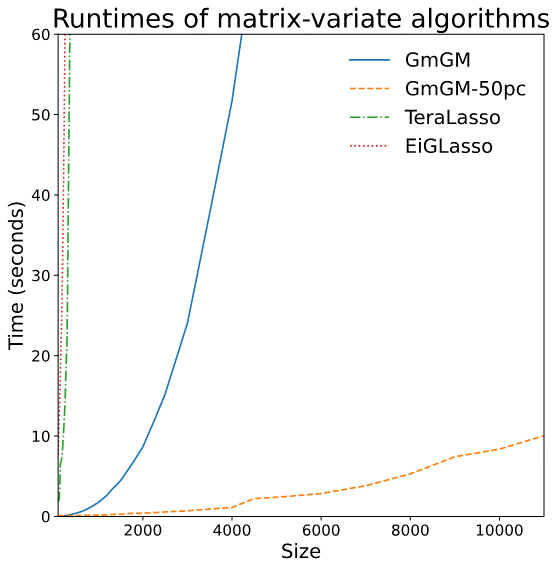
Limitations of prior work
-
Not scalable to millions of features
-
Iterative algorithms
-
Use an eigendecomposition every iteration (O(n^3) runtime - > slow)
-
O(n^2) memory usage
Do we need to scale to Millions of samples?




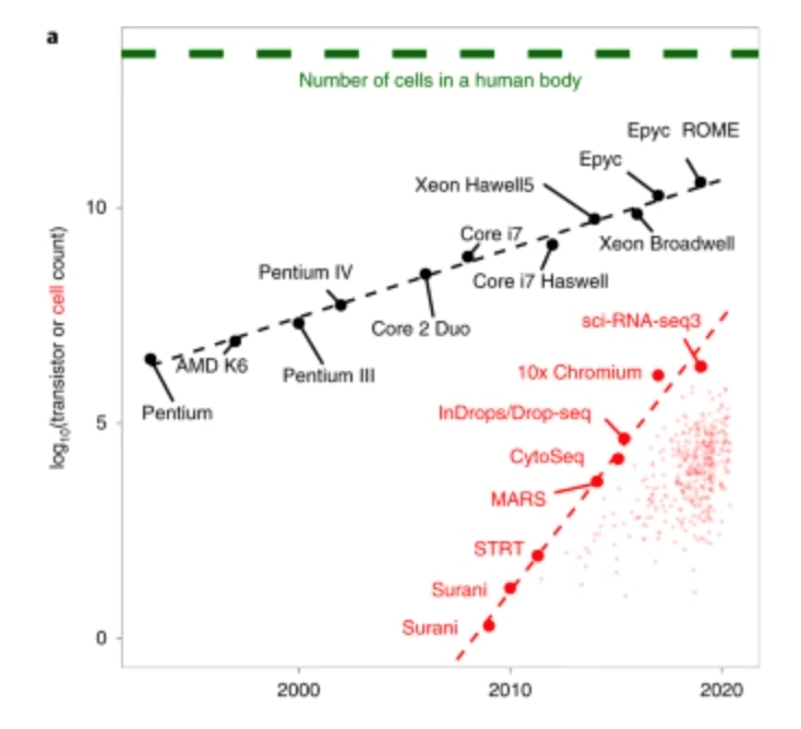
The triumphs and limitations of computational methods for scRNA-seq (Kharchenko, 2021)
Do we need to scale to Millions of samples?
Yes!

Part 2
- A metagenomics matrix of 1000 people x 2000 species
- A metabolomics matrix of 1000 people x 200 metabolites
We may be interested in graph representations of the people, species, and metabolites.
GmGm addresses this problem!
GmGM: a fast Multi-Axis Gaussian Graphical Model ongoing PhD project (Andrew Bailey), AISTAT 2024
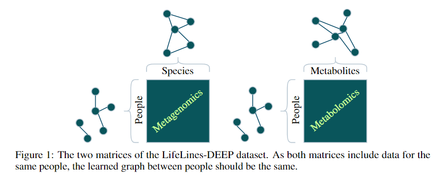
Tensors (i.e. modalities) sharing an axis will be drawn independently from a Kronecker-sum normal distribution and parameterized by the same precision matrix

What is the improvement in GmGM?
In previous work graphical models an L1 penalty is included to enforce sparsity
-
Iterative algorithms
-
Use an eigendecomposition every iteration (O(n^3) runtime-slow!)
If we remove the regularization, we need only 1 eigendecomposition!
In place of regularization, use thresholding


- Syntetic data: runtime plot on a nxn dataset
- Real datasets: Can run on 10,000-cell datasets in well under an hour
Is our GmGM much faster?
- Space complexity: hit the “memory limit” of O(n^2)
- O(n^2) is actually optimal for this problem…
Is our GmGM good enough?

Additional Assumptions!
Work in progress- unpublished
(software available GmGM 0.4.0 )!
Additional Assumptions!
- Both input datasets and precision matrices can be approximated by low-rank versions
- Ensure a fixed upper-bound for the output graph sparsity (i.e. not growing with the dimension of the problem )
- O(n) memory
- O(n^2) runtime
Is our GmGM 0.4.0 much faster / good enough?

Results


Dataset:
157,689 cells
25,184 genes

GmGM VS Prior Work
Memory Use (assuming double-precision)
- Prior Work: ~440 GB
- Ours: ~2 GB
Runtimes
- Prior Work: 2,344 days (Projected based on O(n^3) runtime)
- Ours: 20 minutes


Million-cell dataset?
Million-cell dataset?
Too much memory to fit into Bailey's computer’s 8GB RAM, even when highly sparse
Memory use:
- Prior work: 16 TB
- Ours: depends on sparsity, 20 GB if same level as previous
Runtime:
- Prior work: 1901 years [projected]
- Ours: 15 hours [projected]
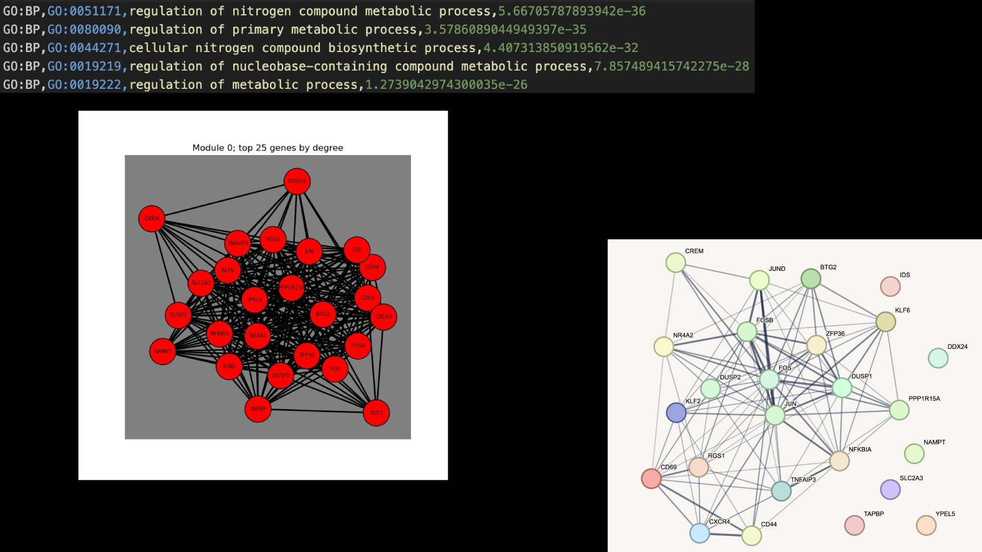
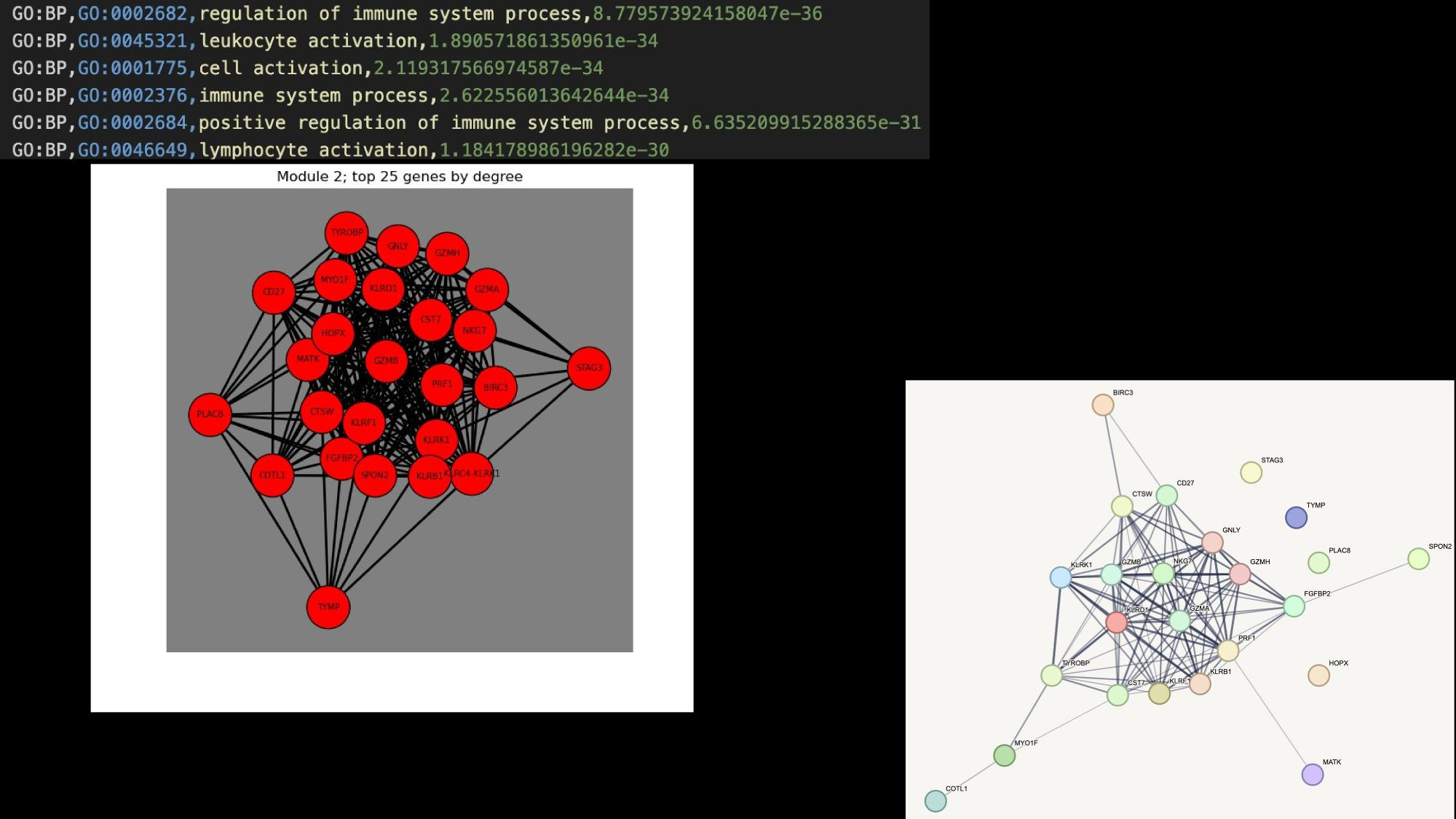
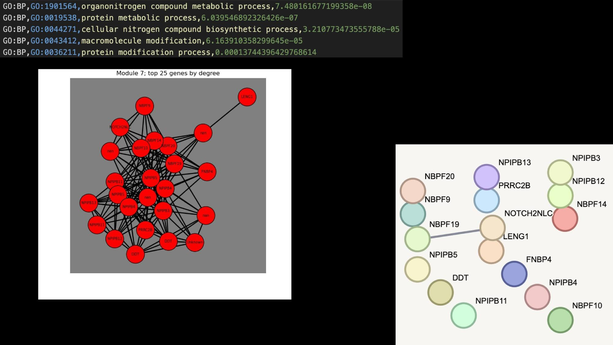
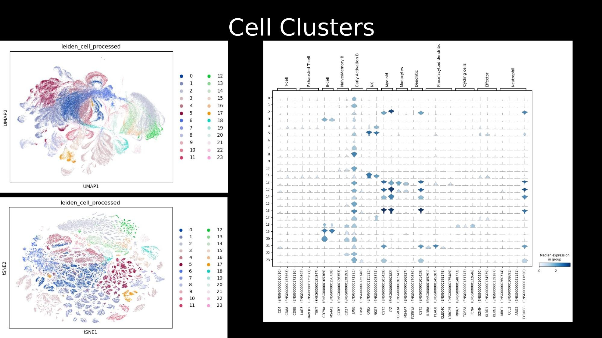
Application Examples

Practical tutorial in github codespaces

Part 3
Instructor: Bailey Andrew, University of Leeds
Ellis_Summer_School2024
By Luisa Cutillo
Ellis_Summer_School2024
- 495


