Gaussian Graphical Models for Multi-Omics Analysis with GmGM
Luisa Cutillo, l.cutillo@leeds.ac.uk, University of Leeds
in collaboration with
Andrew Bailey, and David Westhead, UoL
Outline
- Background on Gaussian Graphical models
- Our Approach:
GmGM

Background on Gaussian Graphical Models (GGM)

What is a GGM?
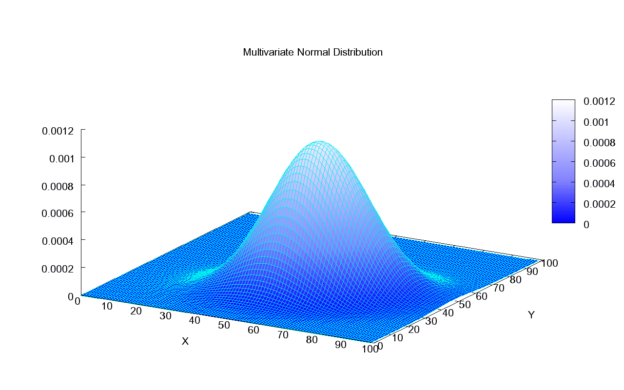
It is just a multivariate Gaussian distribution in !
Precision matrix


p= number of features,
What makes this a Graphical model?
We need to define a graph G(V,E) !

Set of Vertexes V=
Set of Edges E = Precision matrix
Markov Property:
Nodes 1 and 5 are conditionally independent given node 2
Edges correspond to direct interactions between nodes
Partial correlations via
partial correlation
Conditional Independence = SPARSITY!
A hypothetical example of a GGM on psychological variables. (Epskamp at all 2018)
Fatigue
Insomnia
Concentration
(Dempster, 72) it encodes the conditional independence structure
Focus on
Expresses the dependency graph
Example: Random Walk
What is the precision matrix?
About Sparsity...
- We want to study GGMs where is sparse
- This means more conditional independent variables
- Fewer elements to estimate -> Fewer data needed
Sparsity assumption => max graph degree d<<p
is reasonable in many contexts!
Example: Gene interaction networks
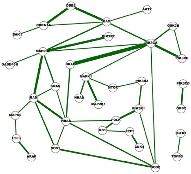
Example: Genes Interaction Networks Inference
- Inference 15 cancer networks and 10 normal networks using The Cancer Genome Atlas (TCGA) RNA-Seq gene expression data and GGM
- Subsets of genes outlined in the KEGG cancer pathways
- Networks were compared to further identify cross-cancer gene interactions.
Fig. 6. A network of strong cross-cancer interactions. Cancer Genetic Network Inference Using Gaussian Graphical Models. (2019) Zhao and Duan.
About Sparsity...
However the " Bet on Sparsity principle" introduced Tibshirani 2001, "In praise of sparsity and convexity":
(...no procedure does well in dense problems!)
- How to ensure sparsity?
Graphical Lasso (Friedman, Hastie, Tibshirani 2008):
imposes an penalty for the estimation of
Limitation
- Assumption of independence between features and samples
- Finds graph only between features
Features
Samples
Data
Main Aim:
Remove the independence assumption
Graph estimation without independence assumption

- Feature independence or data point independence is a model choice issue.
- General framework that models conditional independence relationships between features and data points together.
Deal with estimating a sparse graph that interrelates both features and data points .
-
video data example (Kalaitzis et al., 2013): both the frames (pictures over time) and the image variables (pixels) are correlated.

-
Single cell data: extract the conditional independence structure between genes and cells, inferring a network both at genes level and at cells level.
Cells
Genes
| 2 | ... | 10 |
|---|---|---|
| : | ... | : |
| 5 | ... | 7 |
Graph estimation without independence assumption
Bigraphical lasso: A different point of view
Preserves the matrix structure by using a Kronecker sum (KS) for the precision matrixes
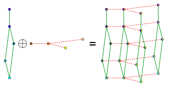

KS => Cartesian product of graphs' adjacency matrix
(eg. Frames x Pixels)

Bigraphical lasso: A different point of view
(kalaitzis et al. (2013))
Limitations:


- Space complexity: There are dependencies but actually implemented to store elements
- Computational time: Very slow, could only handle tens of samples.
We exploit eigenvalue decompositions of the Cartesian product graph to present a more efficient version of the algorithm which reduces memory requirements from O(n^2p^2) to O(n^2+ p^2).
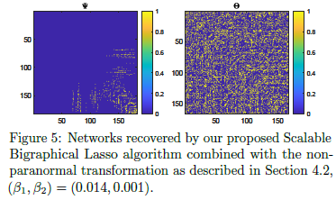
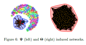
mEST dataset: 182 mouse embryonic stem cells (mESCs) with known cell-cycle phase. We selected a subset of 167 genes involved in the mitotic nuclear division (M phase) as annotated in DAVID database. Buettner et al. (2015)
https://github.com/luisacutillo78/Scalable_Bigraphical_Lasso.git
Two-way Sparse Network Inference for Count Data
S. Li, M. Lopez-Garcia, N. D. Lawrence and L. Cutillo (AISTAT 2022)

Still not good enough!
Improvements of scBiglasso
VS
BigLasso:
-
Memory requirements:
-
Computational Time: from tens of samples to a few hundreds
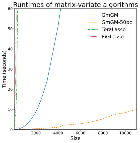
- TeraLasso (Greenewald et al., 2019), EiGLasso (Yoon & Kim, 2020) better space and time complexity (~scLasso)
- Can run on low thousands in a reasonable amount of time
Related work for scalability
Limitations of prior work
-
Not scalable to millions of features
-
Iterative algorithms
-
Use an eigendecomposition every iteration (O(n^3) runtime - > slow)
-
O(n^2) memory usage
Do we need to scale to Millions of samples?




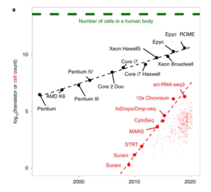
The triumphs and limitations of computational methods for scRNA-seq (Kharchenko, 2021)
Beating Moore’s law.
- number of cells measured by landmark scRNA-seq datasets over years (red),
- increase in the CPU transistor counts (black).
- estimated number of cells in a human body (green dashed line).
Do we need to scale to Millions of samples?
Yes!

- A metagenomics matrix of 1000 people x 2000 species
- A metabolomics matrix of 1000 people x 200 metabolites
We may be interested in graph representations of the people, species, and metabolites.
GmGm addresses this problem!
GmGM: a fast Multi-Axis Gaussian Graphical Model ongoing PhD project (Andrew Bailey), AISTAT 2024
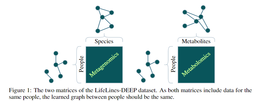
Tensors (i.e. modalities) sharing an axis will be drawn independently from a Kronecker-sum normal distribution and parameterized by the same precision matrix

What is the improvement in GmGM?
In previous work graphical models an L1 penalty is included to enforce sparsity
-
Iterative algorithms
-
Use an eigendecomposition every iteration (O(n^3) runtime-slow!)
If we remove the regularization, we need only 1 eigendecomposition!
In place of regularization, use thresholding


- Syntetic data: runtime plot on a nxn dataset
- Real datasets: Can run on 10,000-cell datasets in well under an hour
Is our GmGM much faster?
- Space complexity: hit the “memory limit” of O(n^2)
- O(n^2) is actually optimal for this problem…
Is our GmGM good enough?

Additional Assumptions!
Work in progress- unpublished
(software available GmGM 0.4.0 )!
Additional Assumptions!
- Both input datasets and precision matrices can be approximated by low-rank versions
- Ensure a fixed upper-bound for the output graph sparsity (i.e. not growing with the dimension of the problem )
- O(n) memory
- O(n^2) runtime
Is our GmGM 0.4.0 much faster / good enough?

Is our GmGM 0.4.0 much faster / good enough?
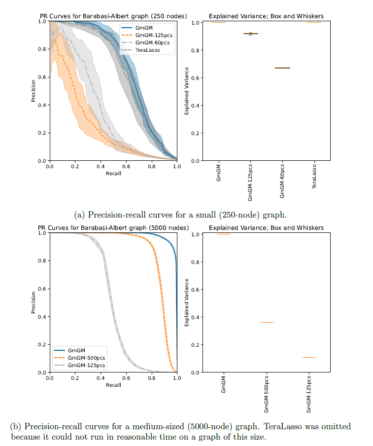
Results


Dataset:
157,689 cells
25,184 genes


GO terms with long names have been replaced with their GO ID; these were all major-histocompatibility-complex-associated GO terms. Immune-related GO terms have been colored blue. These were identified using the Python API of the GProfiler (Kolberg et al., 2023) functional enrichment tool.GmGM VS Prior Work
Memory Use (assuming double-precision)
- Prior Work: ~440 GB
- Ours: ~2 GB
Runtimes
- Prior Work: 2,344 days (Projected based on O(n^3) runtime)
- Ours: 20 minutes


Million-cell dataset?
Million-cell dataset?
Too much memory to fit into Bailey's computer’s 8GB RAM, even when highly sparse
Memory use:
- Prior work: 16 TB
- Ours: depends on sparsity, 20 GB if same level as previous
Runtime:
- Prior work: 1901 years [projected]
- Ours: 15 hours [projected]
Next Steps
- Identification of large gold standards for validation
- Extension to directed networks
- Modelling advancements
Thanks!
ZoomSeminarTuringGroup2024
By Luisa Cutillo
ZoomSeminarTuringGroup2024
- 10


