Beyond Independence: Advances in Network Inference via Gaussian Graphical Models for Multimodal Data
Luisa Cutillo, l.cutillo@leeds.ac.uk, University of Leeds
in collaboration with
Bailey Andrew, and David Westhead, UoL
ELLIS Summer School 2025
Machine Learning for Healthcare and Biology
3 June 2025 - 5 June 2025, University of Manchester
Sections
- Recap: Gaussian Graphical models and GmGM
- New: Non Central GmGM

- Practical tutorial in github codespaces

- New: Strong Product Model
Part 1
Background on Gaussian Graphical Models (GGM) and GmGM
Biological Networks
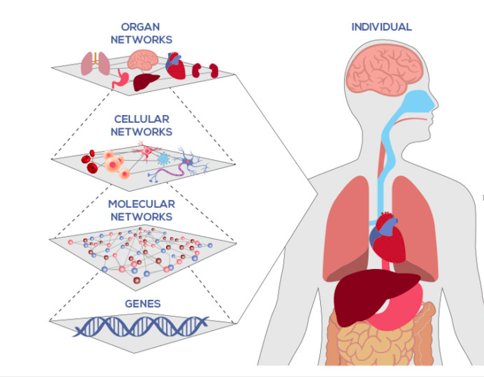
Examples:
- Genetic interaction networks
- Metabolic networks
- Signalling networks
- Gene regulatory networks
- Protein-protein interaction networks
Gaussian graphical model (GGM) estimation is one approach to estimating biological networks
undirected graphical model
X=(X_1,\ldots,X_p)
X1
X3
X2
X4
X5
X6
X7
X8
As
G(V,E)
Vertices V
Edges E
A_{i,j} \neq 0
X_1
X_3
X_5
X_2
X_4
Global Markov Property:
X_A {\mathrel{\perp\!\!\!\perp}} X_B | X_C
conditional independence graph
the absence of an edge between nodes in A and in B corresponds to conditional independence of the random vectors A, B given the separating set C
X=(X_1,\ldots,X_5)
X_1
X_2
X_3
X_4
X_5
What is a GGM?
special case of conditional independence graph where

\Theta=\Sigma^{-1}\in R^{p\times p}
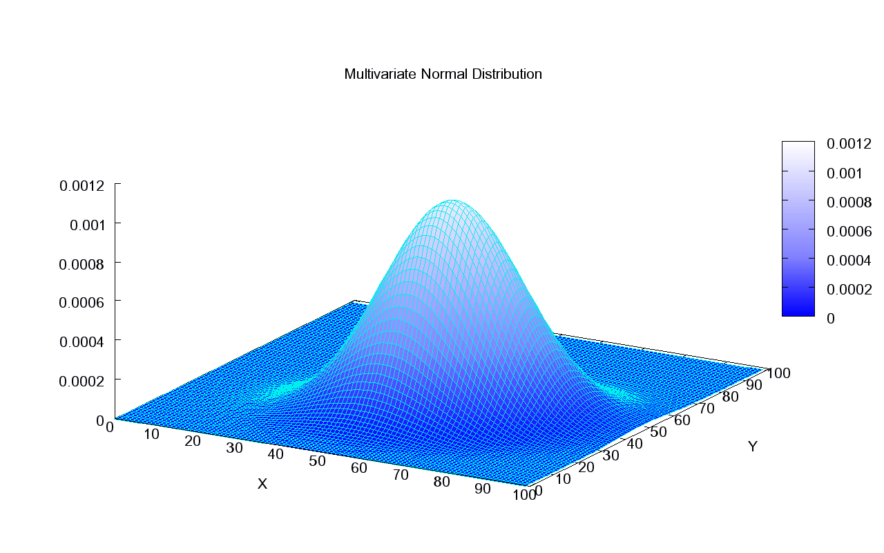
X=(X_1,\ldots,X_p)\sim MVN(\mu, \Sigma)
Edges weights E ∝ Precision matrix
Vertices V
f_x(x_1,\ldots,x_p)\propto exp \left(\frac{(x-\mu)^T\Sigma^{-1}(x-\mu)}{2}\right)
Partial correlations via
partial correlation
\Theta= (\theta_{ij})=\Sigma^{-1}
pcor(i,j)=-\frac{\theta_{i,j}}{\sqrt{\theta_{ii}\theta_{jj}}}
(Dempster, 72) it encodes the conditional independence structure
X_i {\mathrel{\perp\!\!\!\perp}} X_j | X_{-i,-j} \leftrightarrow pcor(i,j)=0
The sparsity pattern of Θ expresses conditional independence relations encoded in the corresponding GGM
Estimating ~ \Theta= (\theta_{ij})=\Sigma^{-1}
0.894
-0.707
correlations: \left[\begin{array}{lll}
\sigma{11}=1 & \sigma{12}=0.894 & \sigma{13}=-0.707\\
\sigma{21}=0.894 & \sigma{22}=1 & \sigma{23}=-0.632\\
\sigma{31}=-0.707 & \sigma{32}=-0.632 & \sigma{33}=1\\
\end{array}\right]
\rho_{i,j}=pcor(i,j)=-\frac{\theta_{i,j}}{\sqrt{\theta_{ii}\theta_{jj}}}
part. \ corr.: \left[\begin{array}{lll}
\rho{11}=1 & \rho{12}=0.816 & \rho{13}= -0.408\\
\rho{21}=0.816 & \rho{22}=1 & \rho{23}=0\\
\rho{31}= -0.408 & \rho{32}=0 & \rho{33}=1 \\
\end{array}\right]
Conditional Independence = SPARSITY!
GGMs Networks VS Correlation Networks
Genes 1, 2, 3
X=(X_1,X2,X_3), e=(e_1,e_2,e_3)\sim_{iid} N(0,1)
X_1=3+e_1,
~ ~X_2=2X_1+e_2,
~ ~ X_3=-X_1+e_3
X_3
X_1
X_2
-0.632
0.816
-0.408
X_3
X_1
X_2
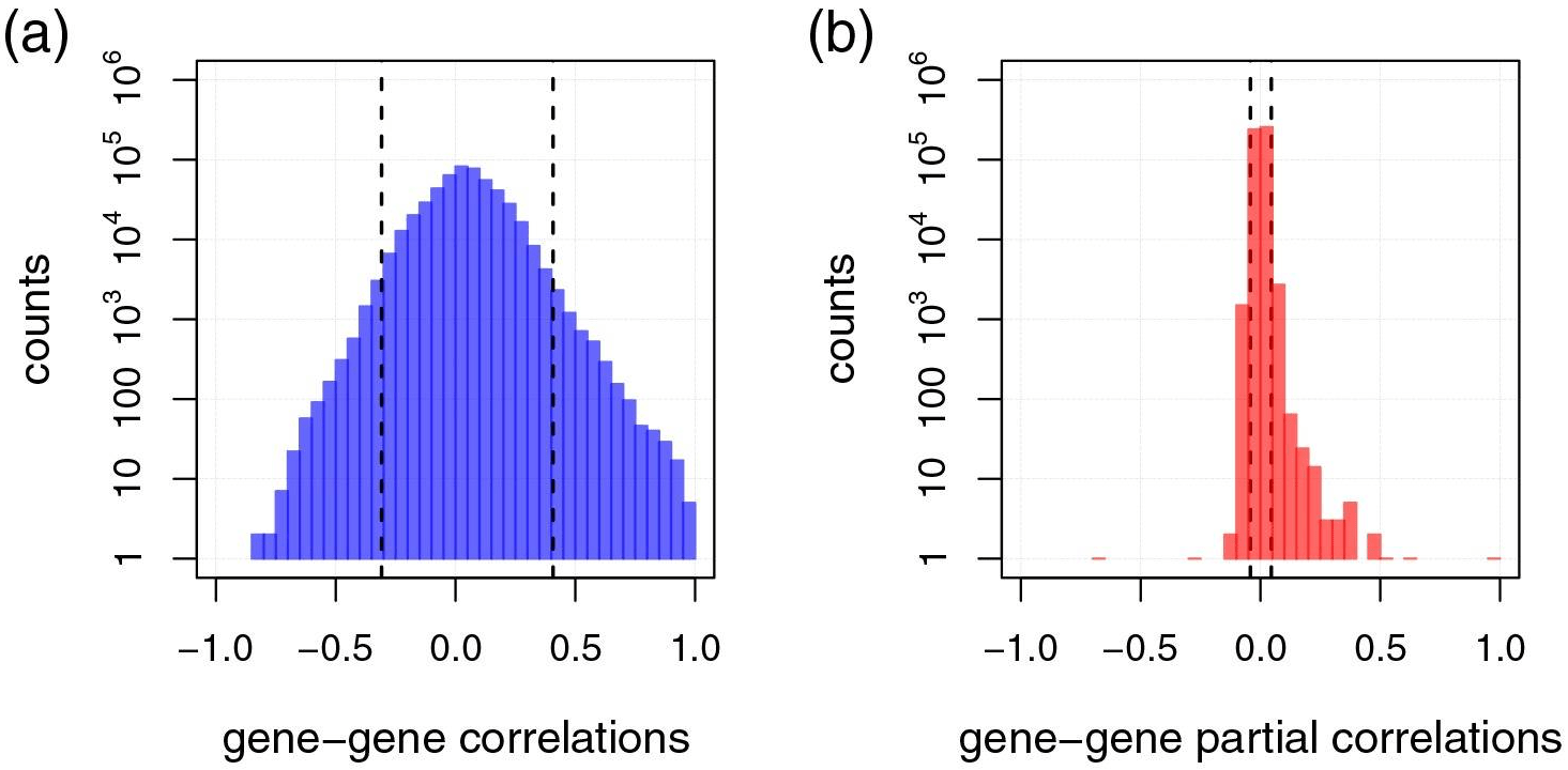
GGMs Networks VS Correlation Networks
IEstimated gene-gene Pearson correlation coefficients (a) with their respective full order partial correlation coefficients (b) for single-cell RNA sequencing data of melanoma metastases (Tirosh et al., 2016).
About Sparsity...
- We want to study GGMs where is sparse
- This means more conditional independent variables
- Fewer elements to estimate -> Fewer data needed
Sparsity assumption => max graph degree d<<p
is reasonable in many contexts!
Example: Gene interaction networks
\Theta
About Sparsity...
However the " Bet on Sparsity principle" introduced Tibshirani 2001, "In praise of sparsity and convexity":
(...no procedure does well in dense problems!)
- How to ensure sparsity?
Graphical Lasso (Friedman, Hastie, Tibshirani 2008):
imposes an penalty for the estimation of
\Theta= \Sigma^{-1}
max_{\Theta>0} \left[ log(det(\Theta))-tr(S\Theta) + \lambda \lVert \Theta \rVert_1 \right]
L_1
Limitation
- Assumption of independence between features and samples
- Finds graph only between features
Features
Samples
Data
Single cell data
extract the conditional independence structure between genes and cells, inferring a network both at genes level and at cells level.
Cells
Genes
| 2 | ... | 10 |
|---|---|---|
| : | ... | : |
| 5 | ... | 7 |
Graph estimation without independence assumption
We need a general framework that models conditional independence relationships between features and data points together.
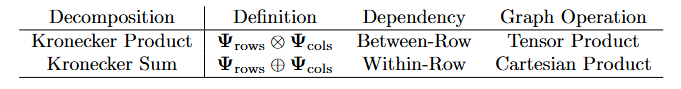
Bigraphical lasso: A different point of view
Preserves the matrix structure by using a Kronecker sum (KS) for the precision matrixes
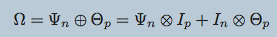
KS => Cartesian product of graphs' adjacency matrix
(eg. Frames x Pixels)

Bigraphical lasso: A different point of view
(Kalaitzis et al. (2013))
Limitations:
- Space complexity: There are dependencies but actually implemented to store elements
O(n^2 + p^2)
O(n^2p^2)
- Computational time: Very slow, could only handle low hundreds samples.
- Exploits eigenvalue decompositions of the Cartesian product graph and a more efficient version of the algorithm
- Reduces memory requirements from O(n^2p^2) to O(n^2+ p^2).
- Replaces Gaussianity with weaker ‘Gaussian copula’ assumption through preprocessing tools non-paranormal skeptic
- Introduces matrix non-paranormal distribution with a Kronecker sum structure
- Can be used on data with arbitrary marginals, as long as relationships between the datapoints ‘behave Gaussianly’).
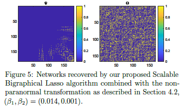
https://github.com/luisacutillo78/Scalable_Bigraphical_Lasso.git
Two-way Sparse Network Inference for Count Data
S. Li, M. Lopez-Garcia, N. D. Lawrence and L. Cutillo (AISTAT 2022)
- TeraLasso (Greenewald et al., 2019), EiGLasso (Yoon & Kim, 2020) better space and time complexity (~scLasso)
- Can run on low thousands in a reasonable amount of time
Related work for scalability
Limitations of prior work
-
Not scalable to millions of features
-
Iterative algorithms
-
Use an eigendecomposition every iteration (O(n^3) runtime - > slow)
-
O(n^2) memory usage
Do we need to scale to Millions of samples?

What is the improvement in GmGM?
In previous work graphical models an L1 penalty is included to enforce sparsity
-
Iterative algorithms
-
Use an eigendecomposition every iteration (O(n^3) runtime-slow!)
If we remove the regularization, we need only 1 eigendecomposition!
In place of regularization, use thresholding

Part 2
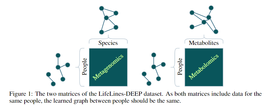
- A metagenomics matrix of 1000 people x 2000 species
- A metabolomics matrix of 1000 people x 200 metabolites
We may be interested in graph representations of the people, species, and metabolites.
GmGm addresses this problem!
GmGM: a fast Multi-Axis Gaussian Graphical Model ongoing PhD project (Andrew Bailey), AISTAT 2024
\begin{align*}
\mathcal{D}^\gamma \sim \mathcal{N}\left(\mathbf{0}, \left(\bigoplus_{\ell\in\gamma}\mathbf{\Psi}_\ell\right)^{-1}\right) &\iff \mathcal{D}^\gamma \sim \mathcal{N}_{KS}\left(\left\{\Psi_\ell\right\}_{\ell\in\gamma}\right)
\end{align*}
Tensors (i.e. modalities) sharing an axis will be drawn independently from a Kronecker-sum normal distribution and parameterized by the same precision matrix
\begin{align*}
\mathbf{D}^\mathrm{metagenomics} \sim& \mathcal{N}_{KS}\left(\mathbf{\Psi}^\mathrm{people}, \mathbf{\Psi}^\mathrm{species}\right) \\
\mathbf{D}^\mathrm{metabolomics} \sim& \mathcal{N}_{KS}\left(\mathbf{\Psi}^\mathrm{people}, \mathbf{\Psi}^\mathrm{metabolites}\right)% \\
%&\text{(independently)}
\end{align*}
Additional Assumptions!
- Both input datasets and precision matrices can be approximated by low-rank versions
Still some limitations:
- the initial eigen-decomposition is O(N^3) per axes anyway
- this can be unfeasible for large and complex datasets
- O(pn) memory
- O(pn^2) runtime
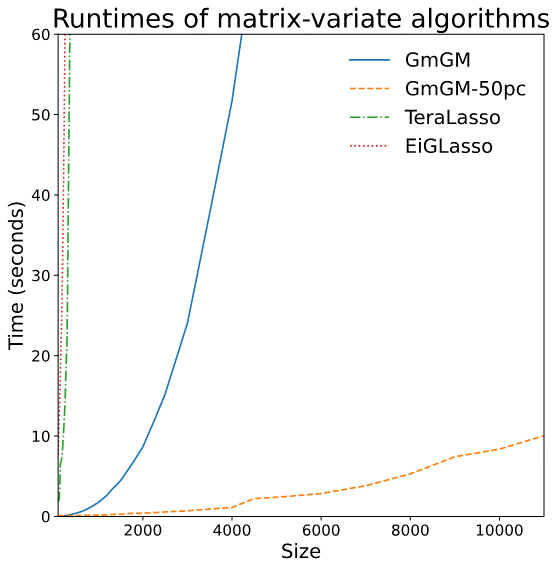
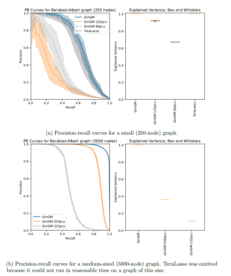
Is our GmGM much faster / good enough?
Is our GmGM much faster / good enough?
Part 2
2025
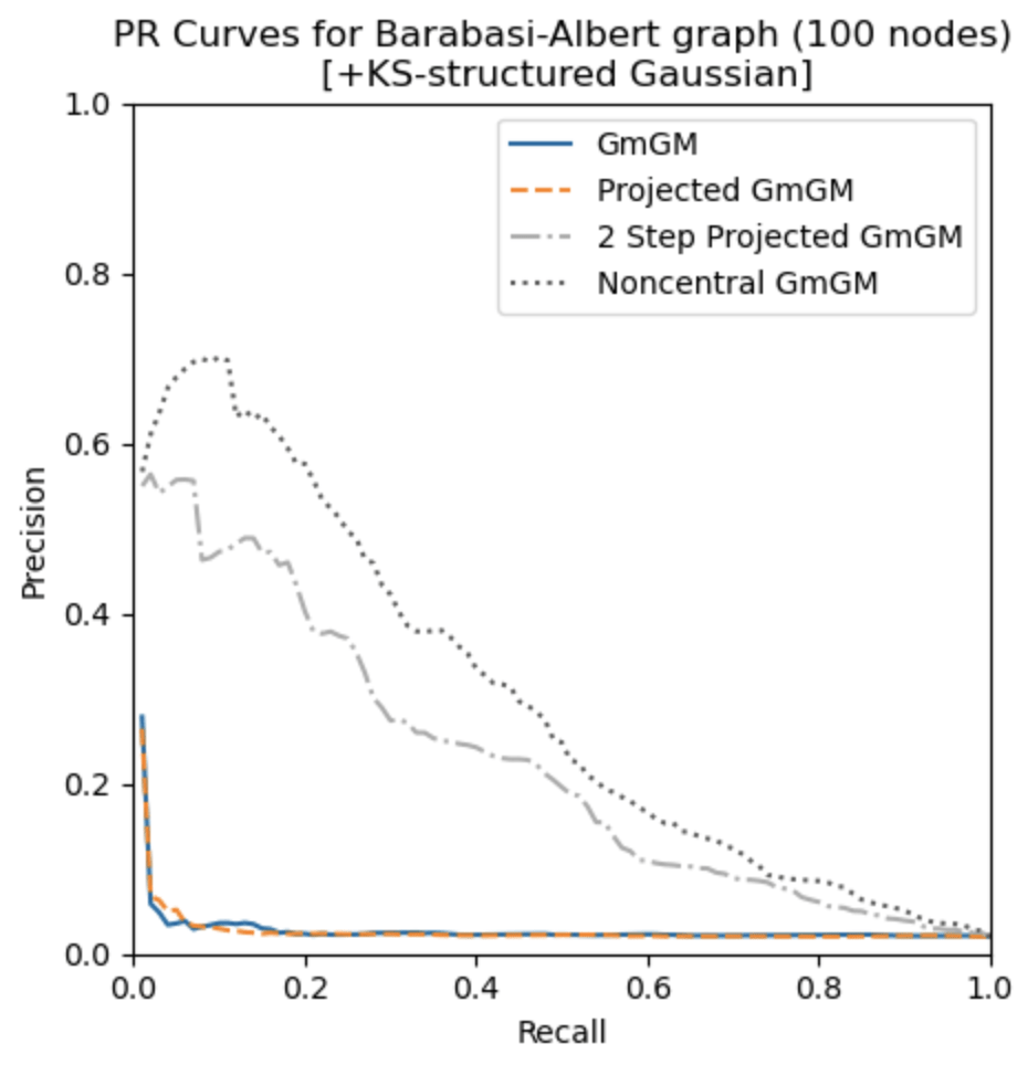
What’s the Problem with Uncentered Data?
In multi-axis case, inference is usually done in a one sample scenario
Zero mean assumption
can cause egregious modelling errors!
We relax the zero-mean assumption
we propose the
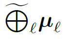
“Kronecker-sum-structured mean”

model with likelihood that
can be solved efficiently with coordinate descent.

Remarks
- noncentral GmGM is a ‘drop-in wrapper’ for pre-existing methods!
- Our estimator for the parameters is the global maximum likelihood estimator
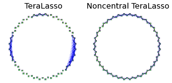
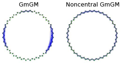
Applying our correction
Part 3
2025
Genes
Cells
| 2 | ... | 10 |
|---|---|---|
| : | ... | : |
| 5 | ... | 7 |
Dependency between genes
Dependency between cells
How do these two types of dependency interact?
X
Y
X
Y
Z
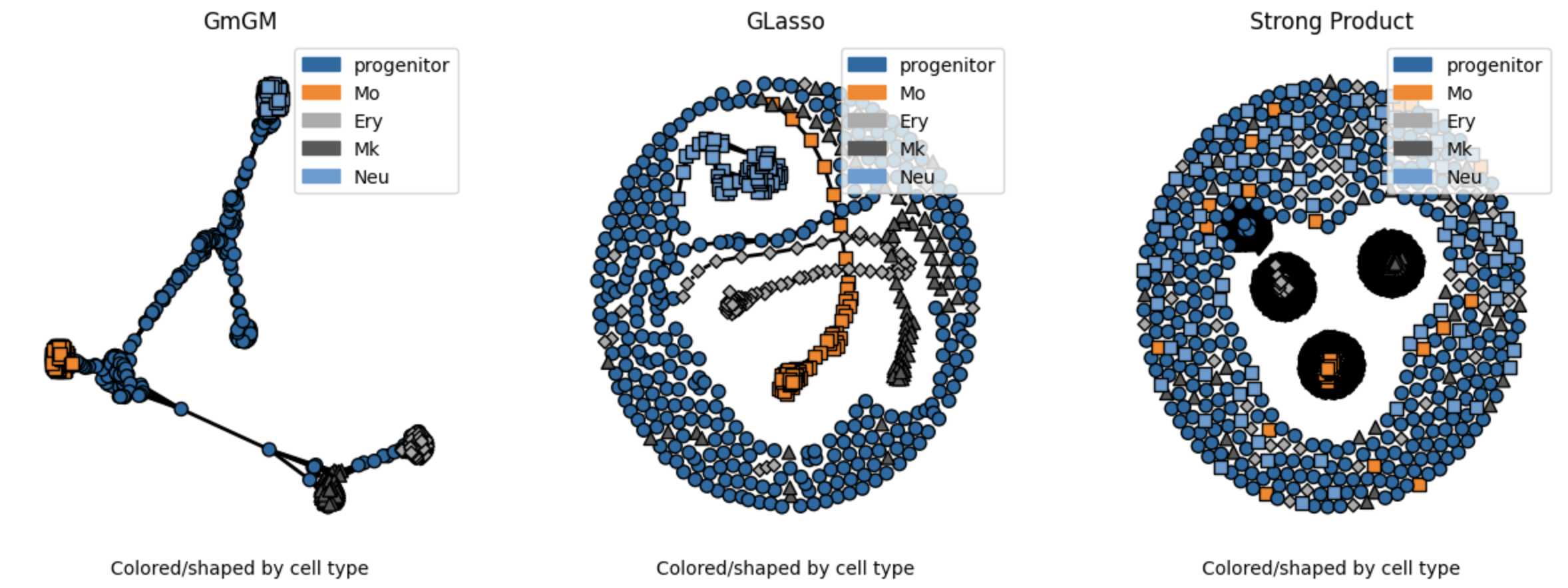
The Strong Product differentiate and learns:
- within-row interaction
- between-row interaction
Model Choices without independence
\mathbf{X} \in R^{d_1\times d_2}, ~ ~ vec[X]\sim N(\mathbf{0},\Omega^{-1})
O(d_1^2d_2^2)
single sample
parameters!
We can impose a specific structure on
\Omega=\zeta(\Psi_{row},\Psi_{cols})
Genes
Cells
| 2 | ... | 10 |
|---|---|---|
| : | ... | : |
| 5 | ... | 7 |
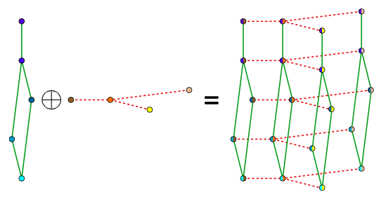
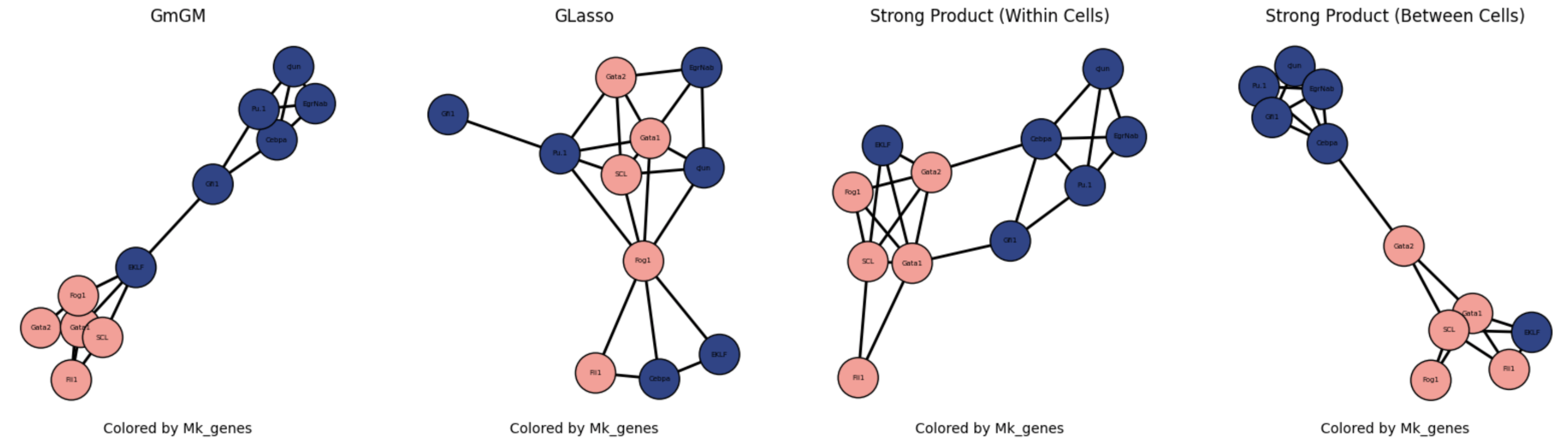
Strong Product model: We add these together!
\mathbf{\Psi}_\mathrm{cells} \otimes \mathbf{I} + \mathbf{I}\otimes\mathbf{\Psi}_\mathrm{genes ~ within ~ cells} + \mathbf{\Psi}_\mathrm{cells}\otimes\mathbf{\Psi}_\mathrm{genes ~ between ~ cells}
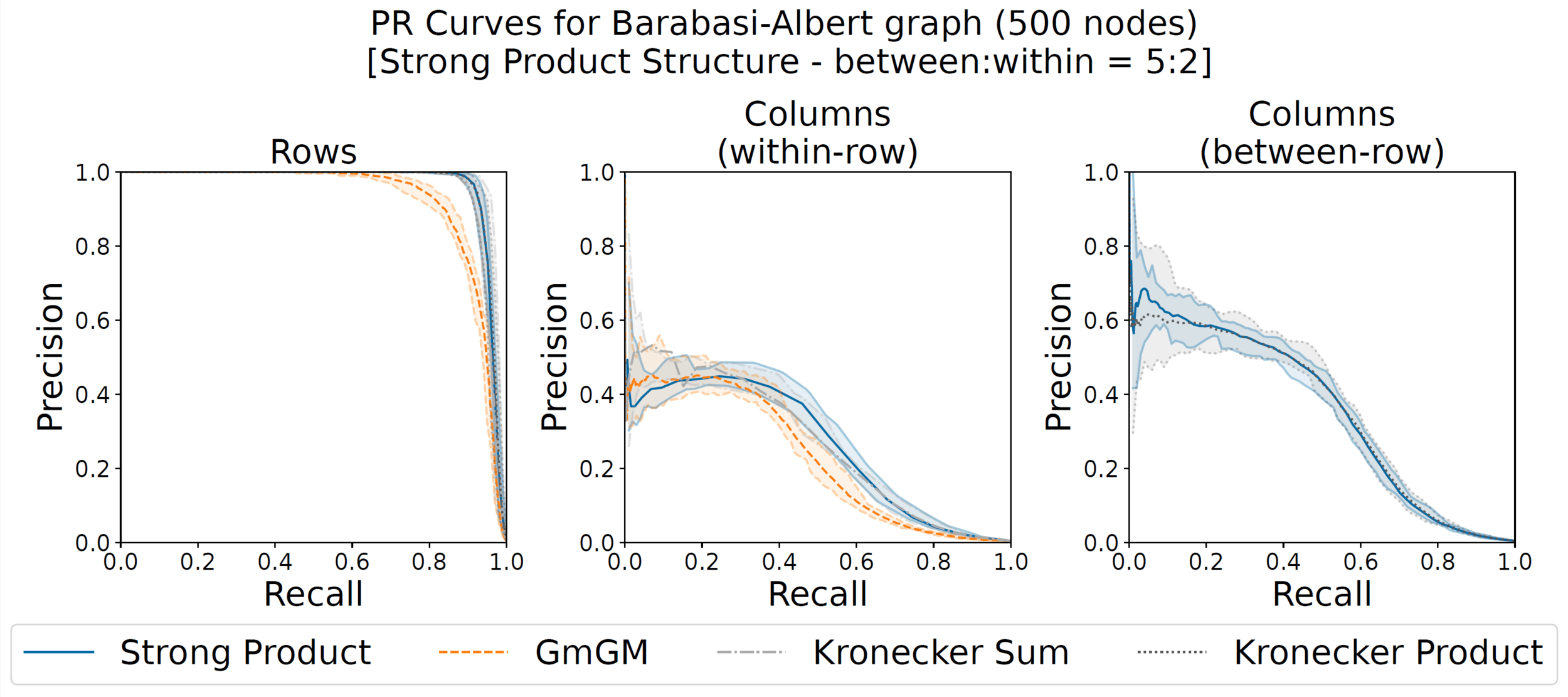
Synthetic data ground truth
(here y=1, x=2.5)
with A, B, C are Barabasi-Albert random graphs with 500 nodes each
y\mathbf{A} \otimes x\mathbf{B} + y\mathbf{A} \oplus \frac{1}{x}\mathbf{C}
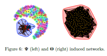
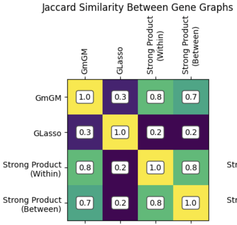
Our Strong Product is the only one that learns both types of column graphs
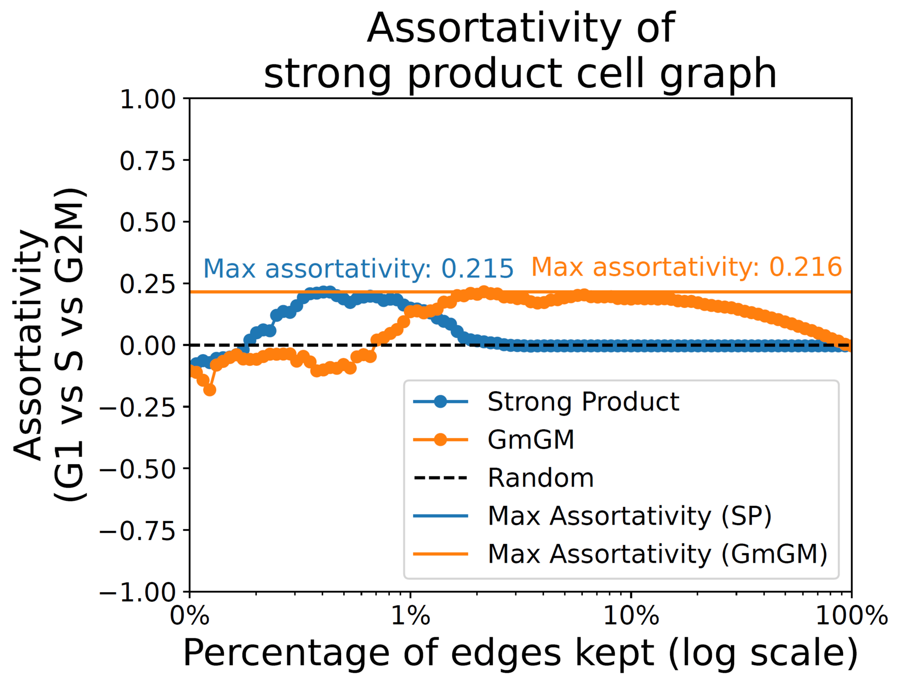
288 mouse embryo stem cell scRNA-seq dataset from Buettner et al. (2015), limited to 167 genes mitosis-related genes cell cycle labelled (G1,S,G2M).
Assortativity:
measures tendency of cells within a stage to connect
1 (tend to connect)
0 (no tendency)
-1 (tend not connect)
Results


Practical tutorial in github codespaces
Part 4
Instructor: Bailey Andrew, University of Leeds
Practical
- Synthetic data (15min)
- Getting the most out of GmGM (15min)
- Real data (15min)
- Open-ended challenges
Ask questions if stuck or curious!
Ellis_Summer_School2025
By Luisa Cutillo


