PV226: Data Exploration
So... what is data exploration?
Takes the most of first phase (60-80%)
Recommended skill:
STATISTICS
1. Step: Get the data
I recommend use data lake and plain CSVs
setup project folder with some meaning full structure
2. Step: Exploratory Analysis
Open CSV in Excel or use Pandas
Identify:
variables
inputs and outputs
data types
import numpy as np
import pandas as pd
import pandas_profiling as pp
from pandas_profiling import ProfileReport

traindf = pd.read_csv('./data/train.csv').set_index('PassengerId')
testdf = pd.read_csv('./data/test.csv').set_index('PassengerId')

traindf.head(3)
Import libs & load csv
boolean
Data Types
categorical
date time
ordinal
categorical
ordinal
Data Types
categorical
ordinal
number
integer
ordinal
float
Data Types
categorical
strings
ordinal
others
Pandas Profiling
the automated way
ProfileReport(train_df, title='Dataset profiling', html={'style':{'full_width':True}})Pandas Describe
basic info
train_df.describe()AutoViz
it will automatically plot charts
from autoviz.AutoViz_Class import AutoViz_Class
AV = AutoViz_Class()

adf=AV.AutoViz(filename="",sep=',', depVar='Survived', dfte=traindf, header=0,
                verbose=2, lowess=False, chart_format='svg',
                max_rows_analyzed=150000, max_cols_analyzed=30)
Univariable analysis
Continuos Variables
Central Tendency: Mean, Median, Mode, Min, Max
Measure of Dispersion: Range, Quartile, Variance, Standard Deviation
Visualization: Histogram, Box Plot
Univariate analysis
Categorical Variables
Count per category
Visualization: bar chart
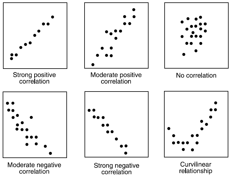
Bivariate analysis
Correlation
Finds strength of relationship
Visualization: matrix/heatmap
We will use Spearman's correlation coefficient
Bivariate analysis
Continuous & Continuous
Visualization: scatter plot
Bivariate analysis
Categorical & Categorical
Visualization: two-way table, stacked column chart
Use chi-square test to derive the statistical significance of relationship
0 = variables are dependent - vs - 1 = variable are independent
Bivariate analysis
Categorical & Continuos
Visualization: box plot
Use Z-Test or T-Test to check statistical significance (T-Test from small number of observations = tens; otherwise Z-Test)
ANOVA for more then 2 groups but this we will keep for stats course
Step 3: Data Cleaning
Missing Values
Solutions:
Detele rows
+ fast and easy
+ good when missing completely at random
- reduces sample size thus model power
Mean/Mode/Median
well...
easy, the most used option
but can be dangerous
Missing Values
Solutions:
Predict/Classify
+ can provide really good results
- if no relationships then poor results
- need to create model
= time consuming
Clustering
+ easier to do then model
+ easy treatment of multiple missing cols
- can be computationally very time consuming
Outliers
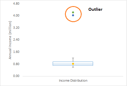
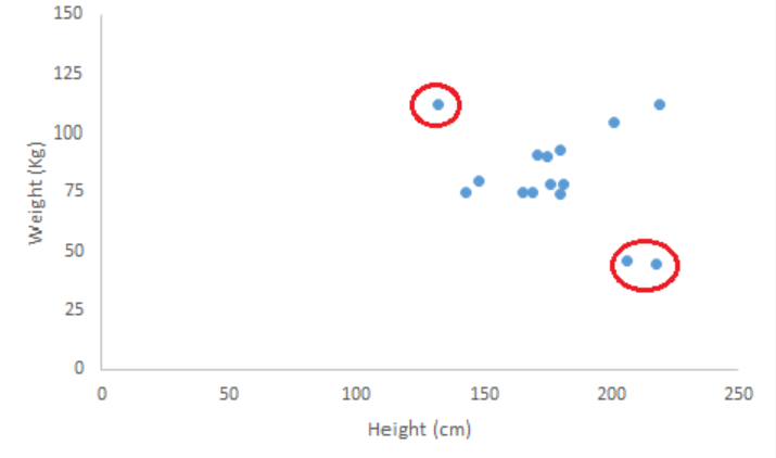
Outliers
Reason: error, non-natural, natural
Human Error
Measurement Error
Experiment Error
Sampling Error
Natural
Outliers
Detection: plots, standard deviation (x3 stddev), Mahalanobis’ distance
Outliers
Solutions:
Delete
+ fast and easy
- but can break model
Transformation
like log
+ easy and can provide good results
- something without result
- does not work on 0
Separate model
+ can provide better results
- more time
- can provide no results at all
Outliers
Solutions:
Binning
transforming to categorical value
Transformation
like square root
+ works on 0
Step 4: Feature Engineering
Adding new variable
eg. add weather data that could affect sales or energy generation
Creating derived variable
fill missing values from other variable, combine some existing variables, apply transformations, change ratios, parse date
Creating dummy variable
Like boolean column per category for categorical feature, tokenize string and so
That can be done manualy
Automatic Option
Use feature tools
import featuretools as ft

es = ft.EntitySet(id = 'titanic_data')
es = es.entity_from_dataframe(entity_id = 'traindf', dataframe = traindf.drop(['Survived'], axis=1),
                              variable_types =
                              {
                                  'Embarked': ft.variable_types.Categorical,
                                  'Sex': ft.variable_types.Boolean,
                                  'Title': ft.variable_types.Categorical,
                                  'Family_Size': ft.variable_types.Numeric,
                                  'LastName': ft.variable_types.Categorical
                              },
                              index = 'PassengerId')

features, feature_names = ft.dfs(entityset = es,
                                 target_entity = 'traindf',
                                 max_depth = 2)
Encode cat features
feature_defs = ['Some column']
feature_matrix_enc, features_enc = ft.encode_features(features, feature_defs)
PV226: Data exploration and cleaning
By Lukáš Grolig


