Visualizing Deep Neural Network Decisions: Prediction Difference Analysis
LuisaMZintgraf, Taco S Cohen, Tameem Adel, MaxWelling
International Conference on Learning Representations 2017
University of Amsterdam, Canadian Institute of Advanced Research, Vrije Universiteit Brussel
15 Feb 2017
Goal
Visualize the response of a deep neural network to a specific input
Related Work
Two approaches for understanding DCNNs through visualization:
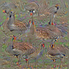
- Find an input image that maximally activates a given node
⇒ visualize what the network is looking for - Visualize how the network responds to a specific input image
⇒ explain a particular classification made by the network
Related Work
Explaining Classifications for Individual Instances
Marko Robnik-Šikonja and Igor Kononenko,
Knowledge and Data Engineering, IEEE Transactions, 2008
Outline
Overview
Approach
Experiment
Conclusion & Future Work
Overview
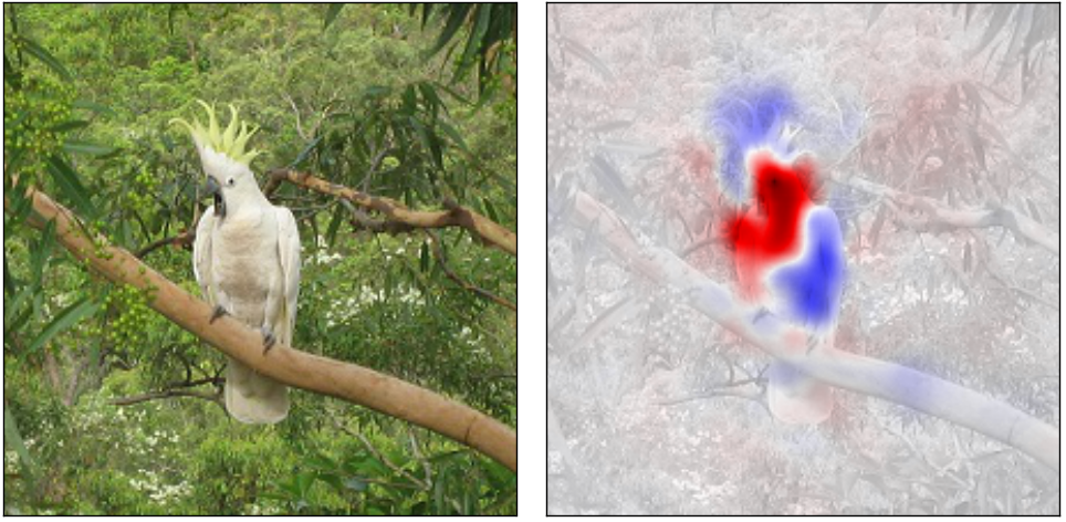
- A new, probabilistically sound methodology for explaining classification decisions made by DNN
- Can be used to produce a saliency map for each instance, node pair
- The map highlights the parts of the input that constitute most evidence for or against the activation of the given node
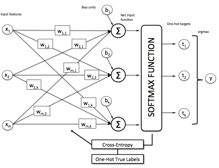
Approach
Prediction Difference Analysis
I
O
I'
O'
1
0
1
1
1
0
1
p(c|\mathbf{x})
p(c|\mathbf{x}_{\backslash i})
Measure how the prediction changes if the feature is unknown
Define:
The probability of O=c given:
\mathbf{x}
all input features
all input features except
x_i
Approach
Prediction Difference Analysis
x_i=p(c|\mathbf{x}) -p(c|\mathbf{x}_{\backslash i})
Relevance of
is easy to compute
How to compute ?
⇒ Simulate the absence of a feature by marginalizing the feature:
p(c|\mathbf{x})
p(c|\mathbf{x}_{\backslash i})
p(c|\mathbf{x}_{\backslash i})=\frac{p(c,\mathbf{x}_{\backslash i})}{p({\mathbf{x}_{\backslash i}})}=\sum_{x_i}\frac{p(c,\mathbf{x}_{\backslash i}, x_i)}{p({\mathbf{x}_{\backslash i}})}
=\sum_{x_i}\frac{p(c,\mathbf{x}_{\backslash i}, x_i)}{p({\mathbf{x}_{\backslash i}},x_i)}\frac{p({\mathbf{x}_{\backslash i}},x_i)}{p({\mathbf{x}_{\backslash i}})}=\sum_{x_i}p(x_i|\mathbf{x}_{\backslash i})p(c|\mathbf{x}_{\backslash i}, x_i)
Approach
Prediction Difference Analysis
p(c|\mathbf{x}_{\backslash i})=\sum_{x_i}p(x_i|\mathbf{x}_{\backslash i})p(c|\mathbf{x}_{\backslash i}, x_i)
How about ? It's infeasible with a large number of features
Assume that is independent of :
p(x_i|\mathbf{x}_{\backslash i})
x_i
\mathbf{x}_{\backslash i}
p(c|\mathbf{x}_{\backslash i})\approx \sum_{x_i}p(x_i)p(c|\mathbf{x}_{\backslash i}, x_i)
is usually approximated by the empirical distribution
(However, an image is not the case)
p(x_i)
Approach
Prediction Difference Analysis
To compare with , we define
Weight of evidence:
\textrm{WE}_i(c|\mathbf{x})=\log_2 (odds(c|\mathbf{x}))- \log_2 (odds(c|\mathbf{x}_{\backslash i}))
p(c|\mathbf{x}_{\backslash i})
p(c|\mathbf{x})
odds(c|\mathbf{x})=\frac{p(c|\mathbf{x})}{1-p(c|\mathbf{x})}
\log_2 (odds(p))
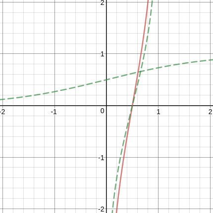
is similar to the inverse of sigmoid function
Avoid 0 probabilities
⇒ Laplace correction:
p \leftarrow \frac{(pN+1)}{N+K}
N: number of training instances
K: number of classes
where
Approach
Prediction Difference Analysis
\textrm{WE}_i(c|\mathbf{x})=\log_2 (odds(c|\mathbf{x}))- \log_2 (odds(c|\mathbf{x}_{\backslash i}))
Positive value:
The feature contributes evidence for the class of interest
⇒ removing it would decrease the confidence of the classifier in the given class
Negative value:
The feature displays evidence against the class
⇒ removing it also removes potentially conflicting or irritating information and the classifier becomes more certain in the investigated class
The feature means of this specific input
x_i
know all the feature know all the features except
x_i
Approach
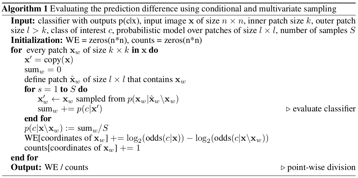
Conditional Sampling
A pixel’s value is highly dependent on other pixels
p(x_i|\mathbf{x}_{\backslash i}) \neq p(x_i)
Two observations:
- A pixel depends most strongly on a small neighborhood around it
- the conditional of a pixel given its neighborhood does not depend on the position of the pixel in the image
Approach
Conditional Sampling
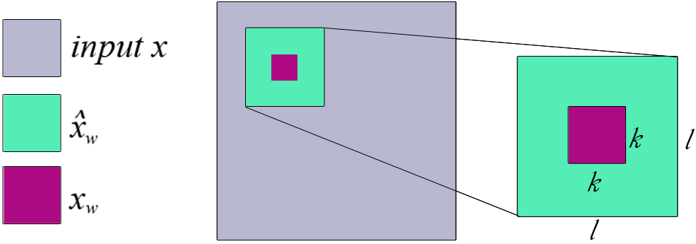
For a pixel , we can find a patch of size that contains , and condition on the remaining pixels in that patch:
p(x_i|\mathbf{x}_{\backslash i}) \approx p(x_i|\hat{\mathbf{x}}_{\backslash i})
x_i
\hat{\mathbf{x}}_{\backslash i}
l
l
x_i
\hat{\mathbf{x}}_{\backslash i}
\hat{\mathbf{x}}_{i}
l \times l
x_i
For a feature to become relevant, it now has to satisfy two conditions:
- Be relevant to predict the class of interest
- Be hard to predict from the neighboring pixels
\uparrow \text{probDiff}_i = p(c|\mathbf{x})-\sum_{x_i}p(x_i|\hat{\mathbf{x}}_{\backslash i})p(c|\mathbf{x}_{\backslash i}, x_i)
Approach
Multivariate Analysis
We expect that a neural network is relatively robust to just one feature of a high-dimensional input being unknown
⇒ remove several features at once:
k \times k
- Do in a sliding window fashion
-
Take the average WE, which is accumulated in the pixel in the overlapping patches
Remove a patch and calculate WEs of pixels in this patch
Approach
Deep Visualization of Hidden Layers
g(z|\mathbf{h}_{\backslash i}) \equiv \mathbb{E}_{p(h_i|\mathbf{h}_{\backslash i})}[z(\mathbf{h})]=\sum_{h_i}p(h_i|\mathbf{h}_{\backslash i})z(\mathbf{h}_{\backslash i},h_i)
We can adapt the method to see how the units of any layer of the network influence a node from a deeper layer
: the vector representation of the output values in a layer H
: the value of a node that depends on
\mathbf{h}
z(\mathbf{h})
\mathbf{h}
We are not dealing with probabilities, so WE is not applicable
Instead, we use activation difference:
\textrm{AD}_i(z|\mathbf{h})=g(z|\mathbf{h})-g(z|\mathbf{h}_{\backslash i})
Approach
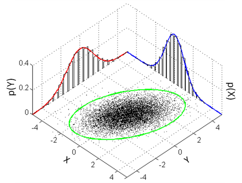
Pseudocode
How to implement it?
Approach
Implementing Conditional Sampling
Idea:
Assume pixels in the patch is a multivariate normal distribution
Implement :
l\times l
- Do statistics on pixels from patches in the training instances
⇒ compute the mean vector and the covariance matrix - Build a multivariate normal model
- Simulate the sampling process from this model
p(\hat{\mathbf{x}}_{w})
Approach
Implementing Conditional Sampling
But we want
⇒ conditional distribution of multivariate normal distribution
l\times l
p(\mathbf{x}_{w}|\hat{\mathbf{x}}_{w}\backslash \mathbf{x}_{w})
proof (an error in the formula of covariance matrix): http://fourier.eng.hmc.edu/e161/lectures/gaussianprocess/node7.html
\hat{\mathbf{x}}_{w}=\begin{bmatrix}
\mathbf{x}_{w}
\\
\hat{\mathbf{x}}_{w}\backslash \mathbf{x}_{w}
\end{bmatrix} = \begin{bmatrix}
\mathbf{x}_{1}
\\
\mathbf{x}_{2}
\end{bmatrix}
\mu=\begin{bmatrix}
\mu_{1}
\\
\mu_{2}
\end{bmatrix}
\Sigma=\begin{bmatrix}
\Sigma_{11} & \Sigma_{12}\\
\Sigma_{21} & \Sigma_{22}
\end{bmatrix}
\mu_{1|2}=\mu_1+\Sigma_{12}\Sigma_{22}^{-1}(\mathbf{x}_2-\mu_2)
\Sigma_{1|2}=\Sigma_{11}+\Sigma_{12}\Sigma_{22}^{-1}\Sigma_{21}
Draw samples from distribution
\textrm{N}(\mu_{1|2}, \Sigma_{1|2})
Experiment
Two parts:
- ImageNet dataset, DCNNs
- MRI scans, logistic regression classifier
Sampling method
- Marginal sampling: empirical distribution
- Conditional sampling: multivariate normal distribution
- Draw only 10 samples
(since no significant difference was observed with more samples)
Experiment
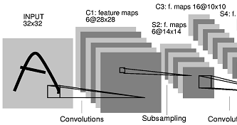
ImageNet: Understanding How a DCNN Makes Decisions
Use images from the ILSVRC challenge:
a large dataset of natural images from 1000 categories
Three DCNNs, use pre-trianed models, implemented by caffe
Analysis time:
- AlexNet: 20 mins/image
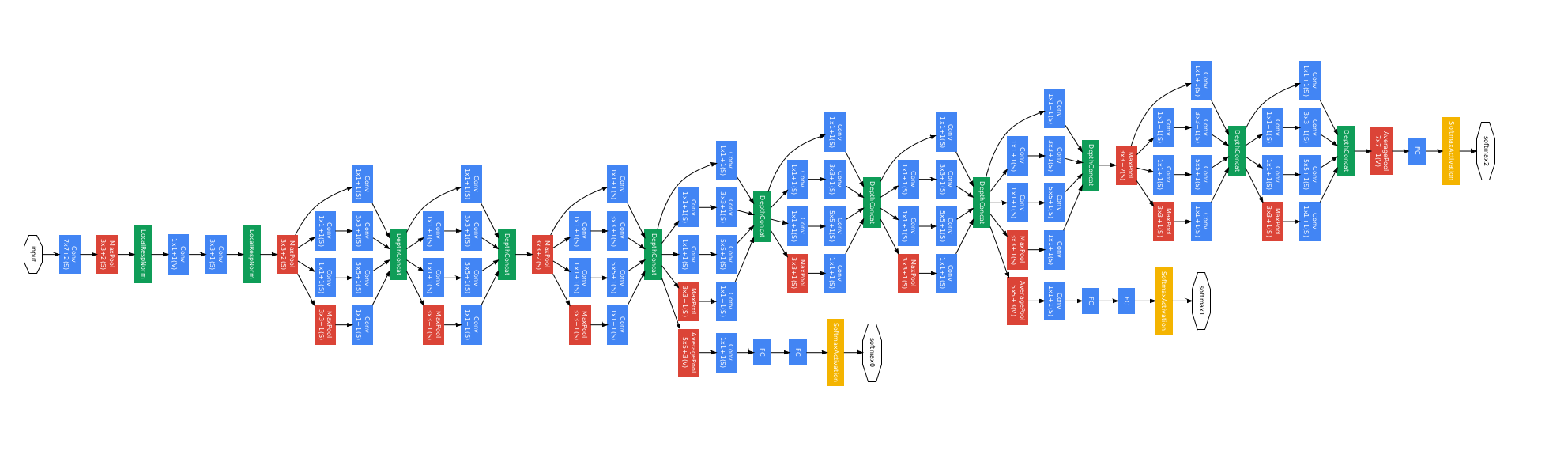
- GoogLeNet: 30 mins/image
- 16-layer VGG Net: 70 mins/image
Experiment
Marginal v.s. Conditional Sampling
For the rest of our experiments, we show results using conditional sampling only
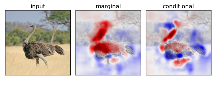
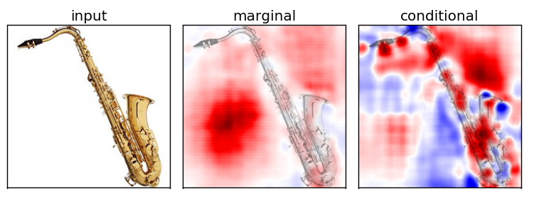
k=10,\ l=14 \ \textrm{GoogLeNet}
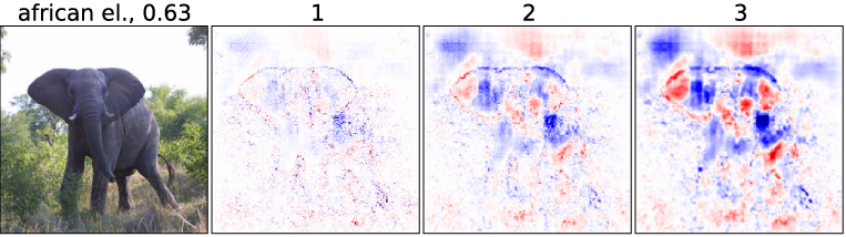
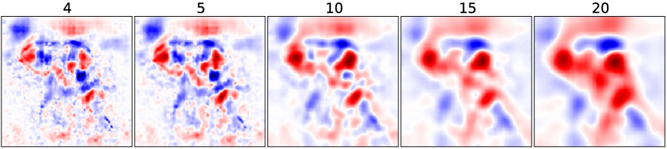
Experiment
Multivariate Analysis
k,\ l=k+4
Experiment
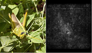
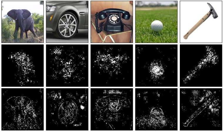
Comparison with Sensitivity Map
- top 5% relevant pixels by the absolute value (in a boolean mask)
- k=1, l=5
- highest scoring class in the penultimate layer
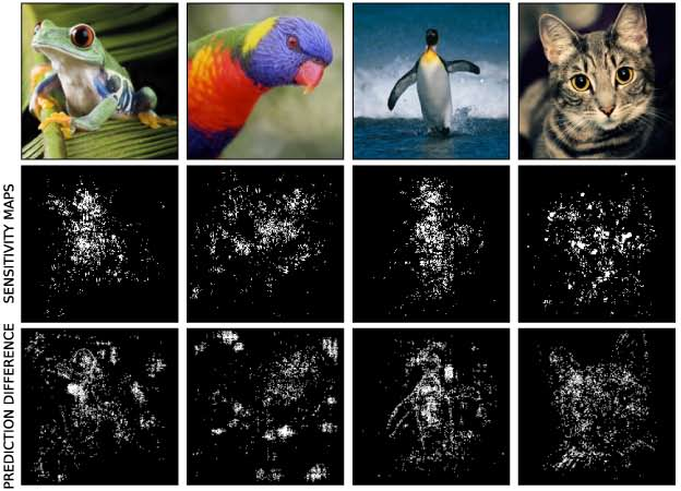
Experiment
Comparison with Sensitivity Map
Experiment
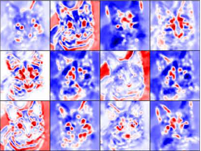
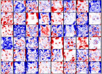
Deep Visualization of Hidden Network Layers
For each feature map in a convolutional layer:
- First, compute the relevance of the input image for each hidden unit in that map
- To estimate what the feature map as a whole is doing, we show the average of the relevance vectors over all units in that feature map
Experiment
Deep Visualization of Hidden Network Layers
Simple image filters
Experiment
Deep Visualization of Hidden Network Layers
specialized to higher level features
Experiment
Deep Visualization of Hidden Network Layers
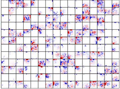
units are highly specialized
Experiment
Deep Visualization of Hidden Network Layers
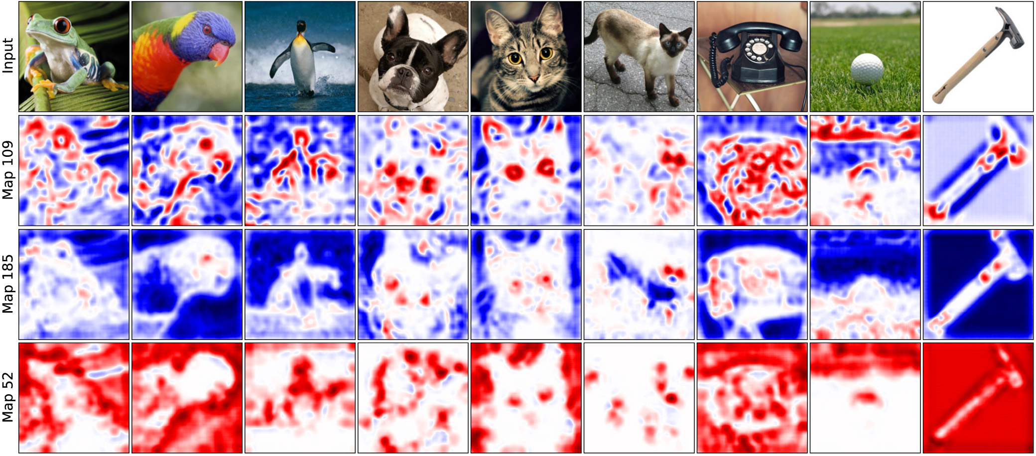
Same layer, different input image
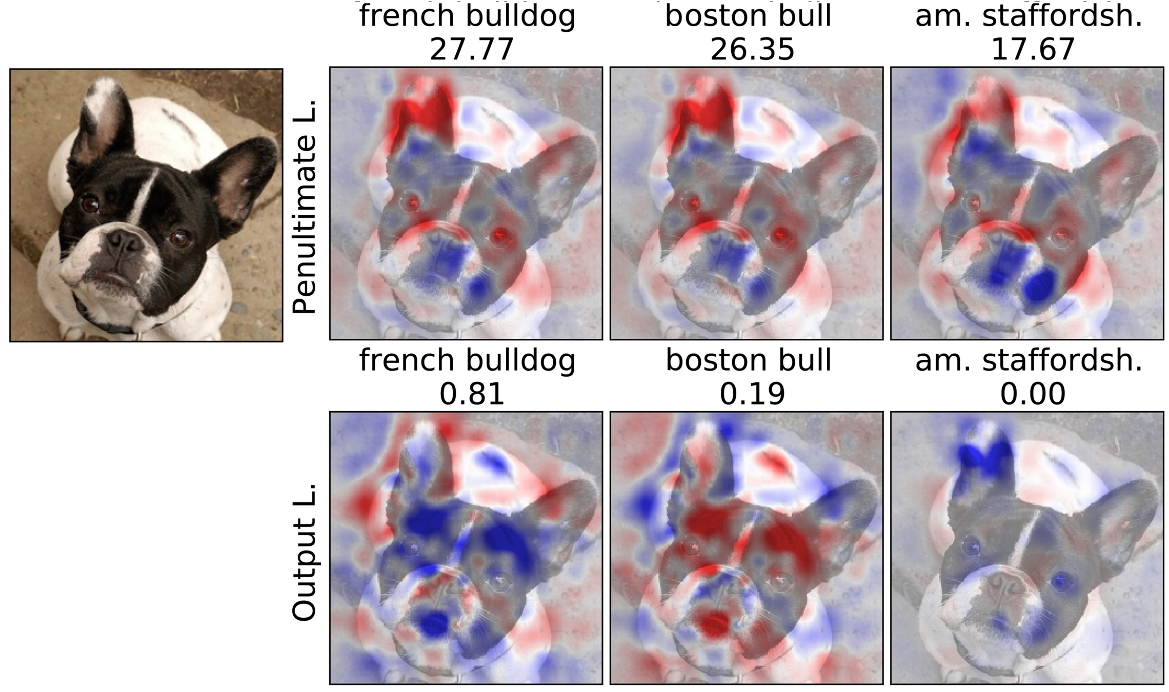
Experiment
Penultimate v.s. Output Layer
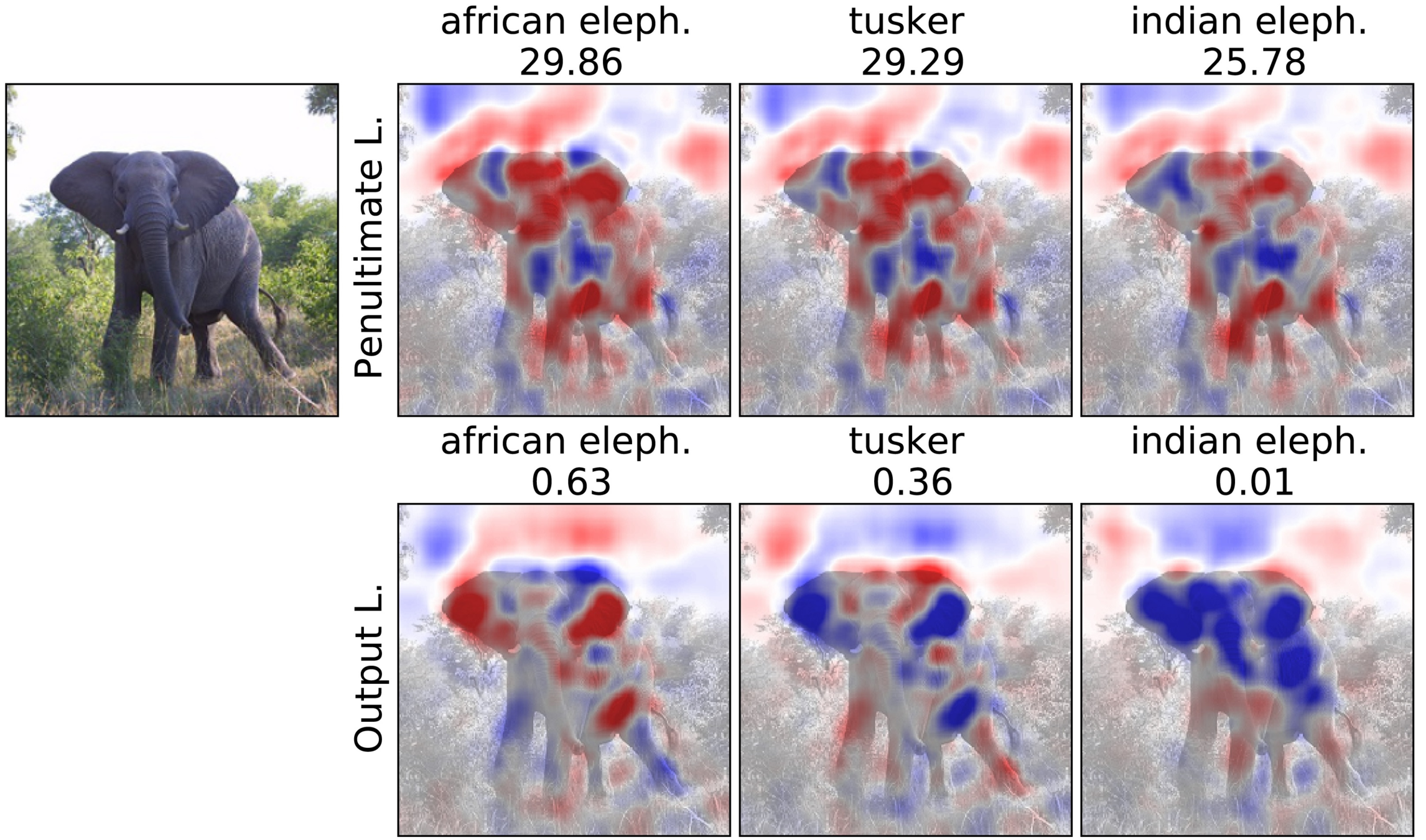
Experiment
Penultimate v.s. Output Layer
Experiment
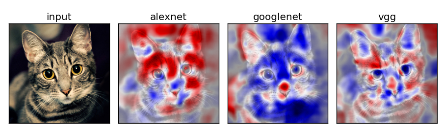
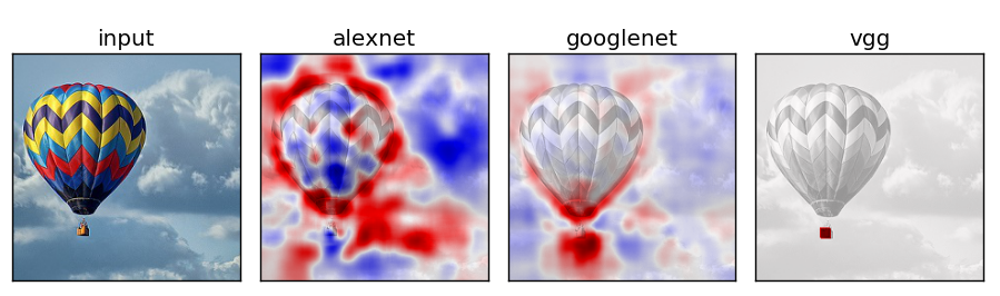
Network Comparison
Experiment
MRI Data: Explaining Classifier Decisions in Medical Imaging
When classifying a patient, the practitioner weigh this information and incorporate it into the overall diagnosis process
MRI dataset of HIV and healthy patients
- COBRA dataset: 3D MRIs from 100 HIV / 70 healthy individuals
- Preprocessing ⇒ Fractional Anisotropy (FA) maps
- Train on slices 29-40, first 70 samples of the HIV classes
L2-regularized Logistic Regression classifier (model details unknown)
- k=3, l=7, adding location information
- 69.3% accuracy in 10-fold cross-validation
- 1.5 hrs/image analysis
Experiment
MRI Data: Explaining Classifier Decisions in Medical Imaging
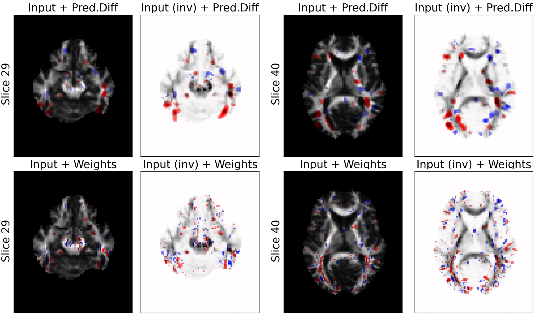
weights of the logistic regression classifier
(noisier, scattered)
prediction difference
Relevance values are shown only for voxels with value above 15% of the absolute maximum value
Experiment
MRI Data: Explaining Classifier Decisions in Medical Imaging
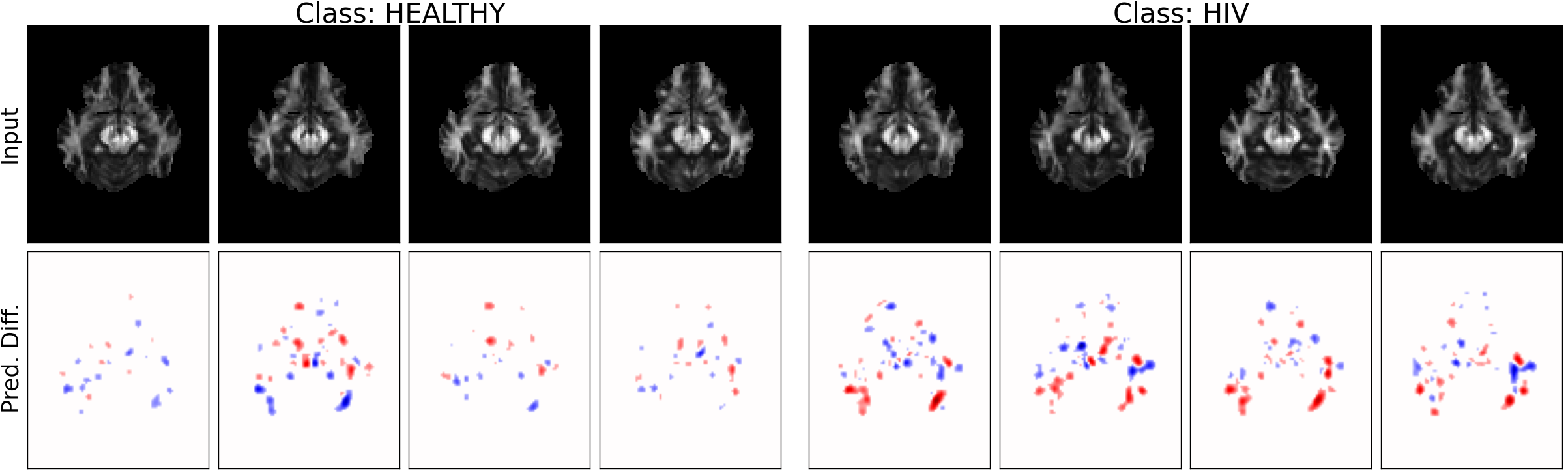
Different class
Experiment
MRI Data: Explaining Classifier Decisions in Medical Imaging
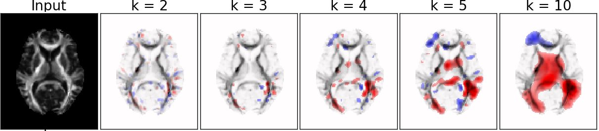
Different patch size
Conclusion & Future Work
Future work
- Try to improve by taking more image information
- Make the method applicable for clinical analysis and practice
a better classification algorithm is required - An interactive 3D visualization model will improve the usability of the system
Contributions
- Conditional sampling
- Multivariate analysis
- Deep visualization
p(x_i|\mathbf{x}_{\backslash i}) \approx p(x_i|\hat{\mathbf{x}}_{\backslash i})
Visualizing Deep Neural Network Decisions: Prediction Difference Analysis
By Maeglin Liao


