Video Frame Synthesis using Deep Voxel Flow
Ziwei Liu, Xiaoou Tang, Raymond Yeh, Yiming Liu, Aseem Agarwala
The Chinese University of Hong Kong, University of Illinois at Urbana-Champaign, Google Inc.
2017, Feb 8
Goal
Frame Interpolation/Extrapolation
Application
- Slow-motion effect
- Increase frame rate

Optical Flow


(\Delta x,\Delta y)
compute flow
on each pixel
Related Work
CNN Approach
- Predict optical flow
Traditional Approach
- Estimate optical flow between frames
- Interpolate optical flow vector
⇒ Optical flow must be accurate
⇒ Require supervision (flow ground-truth)
- Directly hallucinate RGB pixel values
⇒ Blurry
Outline
Overview
Formulation
Refinement and Extension
Experiment
Summary
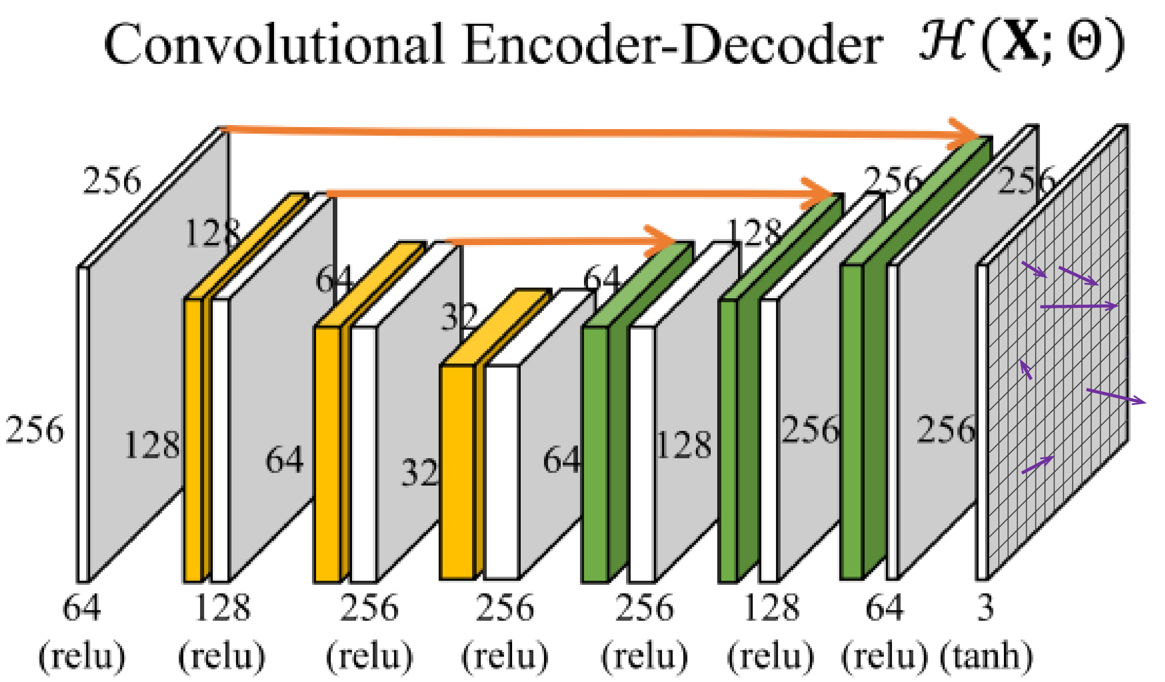
Overview
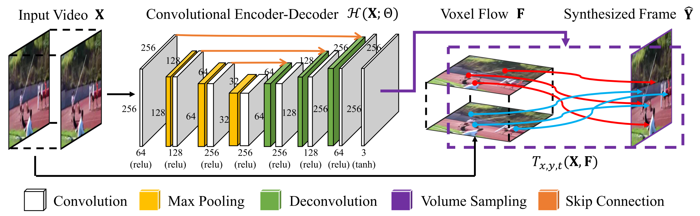
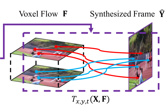
Deep Voxel Flow
Combine the strengths of traditional and CNN approaches
- CNN ⇒ voxel flow
- Volume sampling layer(blending) ⇒ synthesized frame
- Synthesized frame ⇔ ground-truth frame
*voxel=volume pixel=3D pixel
End-to-end trained deep network
No FC layer ⇒ any resolution
Quantitatively and qualitatively improve upon the state-of-the-art
Formulation
Architecture
Y\in \mathbb{R} ^{H\times W}
X\in \mathbb{R} ^{H\times W\times L}
Input frames
Target frame
\hat{Y}\in \mathbb{R} ^{H\times W}
Synthesized frame
F=\mathcal{H}\left( X;\Theta \right) =(\Delta x,\Delta y,\Delta t)
Formulation
CNN ⇒ Voxel Flow
Predict the voxel flow on every pixel of
\Theta
network parameters
Voxel Flow
*Deconvolution
kernel sizes:
5x5, 5x5, 3x3, 3x3, 3x3, 5x5, 5x5
F_{motion}=(\Delta x, \Delta y)
F_{mask}=(\Delta t)
\hat{Y}
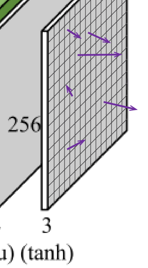
\Delta x, \Delta y, \Delta t \in (-1, 1)
\Delta t \in (0, 1)
it should be:
Formulation
Volume Sampling Layer ⇒ Synthesized Frame
F_{motion}=(\Delta x, \Delta y)
F_{mask}=(\Delta t)
Assume optical flow is temporally symmetric around the in-between frame
Corresponding locations in:
- Previous frame
- Next frame
L^0=(x-\Delta x, y-\Delta y)
L^1=(x+\Delta x, y+\Delta y)
*(x,y):pixel location in the synthesized frame
Linear blending weight between the previous and next frames
Formulation
Volume Sampling Layer ⇒ Synthesized Frame
F_{motion}
F_{mask}
Y
Formulation
Volume Sampling Layer ⇒ Synthesized Frame
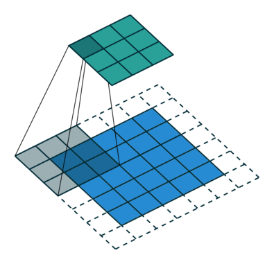
\hat{Y}(x,y)=\sum _{i,j,k\in \left[ 0,1\right] }W^{ijk}X\left( V^{ijk}\right)
Trilinear interpolation
V^{000}=(\lfloor L^0_x\rfloor,\lfloor L^0_y \rfloor,0)
V^{100}=(\lceil L^0_x\rceil,\lfloor L^0_y \rfloor,0)
V^{011}=(\lfloor L^1_x\rfloor,\lceil L^1_y \rceil,1)
V^{111}=(\lceil L^1_x\rceil,\lceil L^1_y \rceil,1)
\ldots
W^{000}=(\lceil L^0_x\rceil-L^0_x)(\lceil L^0_y\rceil-L^0_y)(1-\Delta t)
W^{100}=(L^0_x-\lfloor L^0_x\rfloor)(\lceil L^0_y\rceil-L^0_y)(1-\Delta t)
W^{011}=(\lceil L^1_x\rceil-L^1_x)(L^1_y-\lfloor L^1_y \rfloor)\Delta t
W^{111}=(L^1_x-\lfloor L^1_x\rfloor)(L^1_y-\lfloor L^1_y \rfloor)\Delta t
\ldots
Volume Sampling Function
\mathcal{T}_{x,y,t}(X,\mathcal{H}\left( X;\Theta \right) )=\hat{Y}
Formulation Visualization
Synthesize frame in 1D
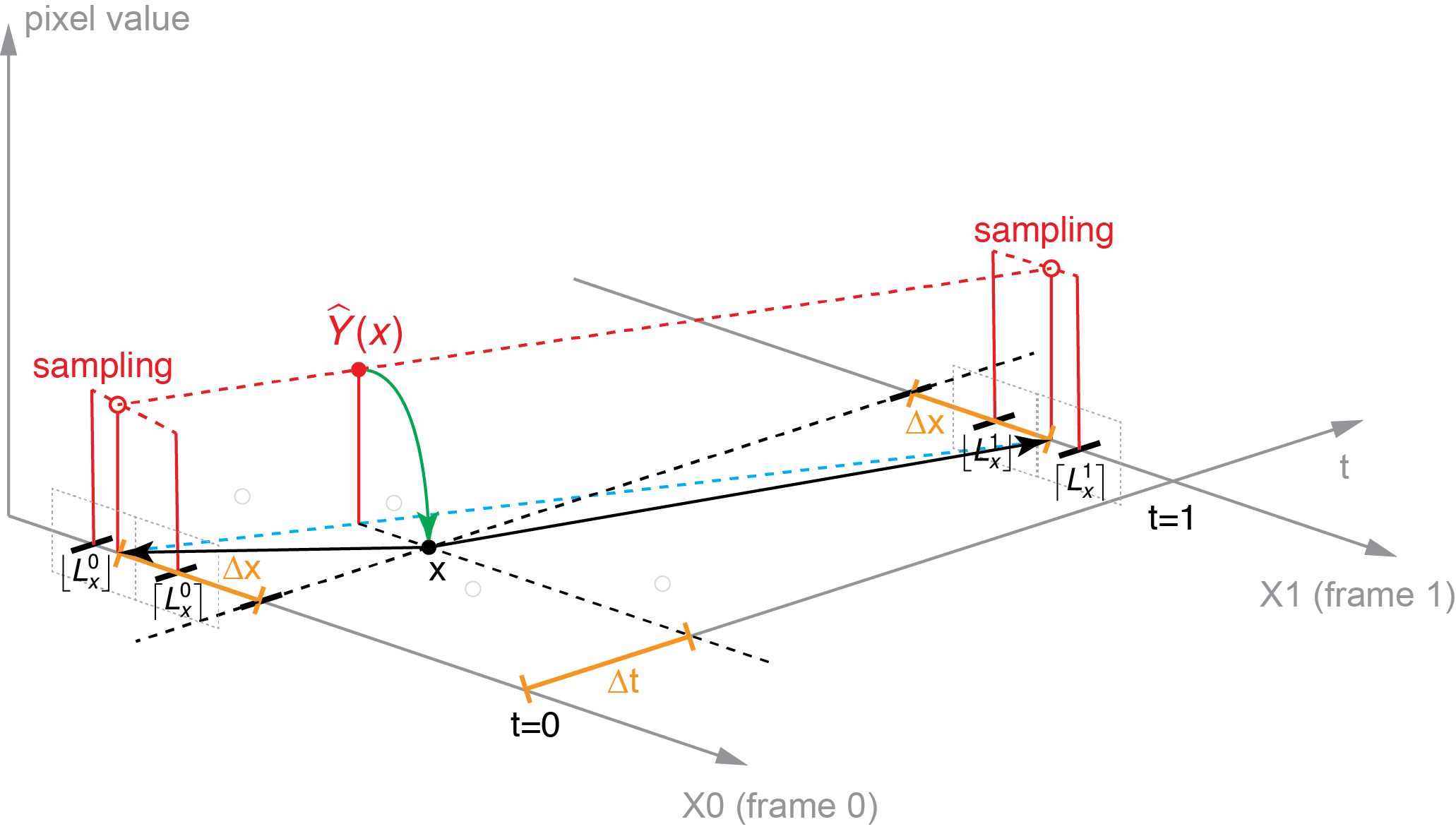
\hat{Y}(x)=\sum _{i,j\in \left[ 0,1\right] }W^{ij}X\left( V^{ij}\right)
Formulation Visualization
Synthesize frame in 2D
\hat{Y}(x,y)=\sum _{i,j,k\in \left[ 0,1\right] }W^{ijk}X\left( V^{ijk}\right)
Digression
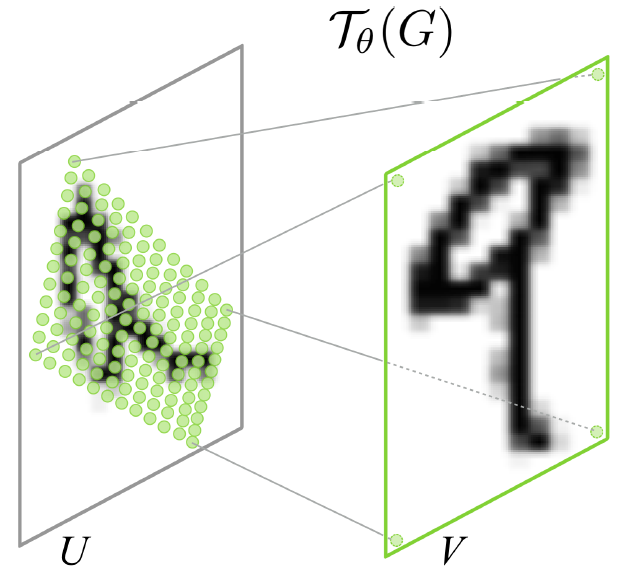
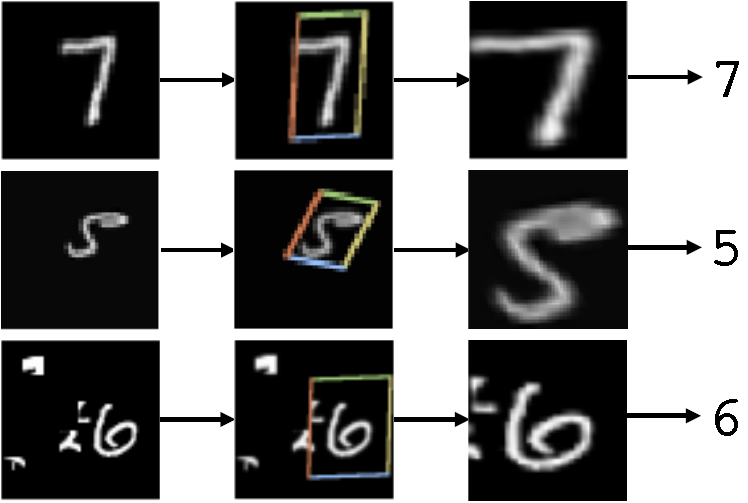
Spatial Transformer Networks
DeepMind, 2015 NIPS, Cited by 222
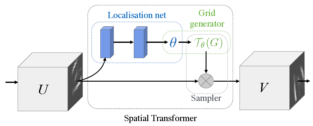
\begin{pmatrix}
x^s_i\\
y^s_i
\end{pmatrix}=\mathcal{T}_{\theta}(G_i)=\begin{bmatrix}
\theta_{11} & \theta_{12} & \theta_{13}\\
\theta_{21} & \theta_{22} & \theta_{23}
\end{bmatrix}\begin{pmatrix}
x^t_i\\
y^t_i\\
1
\end{pmatrix}
Formulation
Synthesized Frame ⇔ Ground-Truth Frame
Loss Function
\dfrac {1} {N}\sum _{\left\langle X,Y\right\rangle \in \mathcal{D}}\left(\left\| Y-\hat{Y} \right\| _{1} + \lambda _{1}\left\| \nabla F_{motion}\right\|_{1}+\lambda_{2}\left\| \nabla F_{mask}\right\|_{1}\right)
total variation:
\sum _{n}\left| x_{n+1}-x_{n}\right|
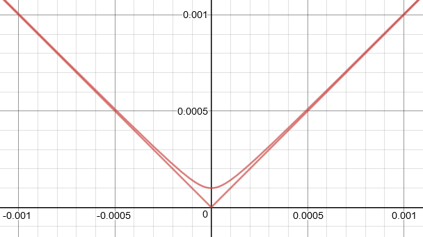
L1 approximated by Charbonnier loss
{\Phi }\left( x\right) =\left( x^{2}+\epsilon ^{2}\right) ^{1 / 2}
Empirically
\lambda_1=0.01
\lambda_2=0.005
\epsilon=0.001
Learning settings
- Batch size: 32
- Batch normalization
- Gaussian init:
- ADAM solver:
\sigma=0.01
lr=0.0001,\beta_1=0.9,\beta_2=0.999
Formulation
End-to-end Fully Differentiable System
\dfrac {d\hat {Y}} {d\Theta }=\dfrac {d\hat {Y}} {dF}\dfrac {dF} {d\Theta }\ \Rightarrow \ \dfrac {\partial \hat {Y}\left( x,y \right) } {\partial \left( \Delta x\right) }=\sum _{i,j,k\in \left[ 0,1\right] }E^{ijk}X\left( V^{ijk}\right)
=\sum _{t\in \left[ 0,1\right] }\sum _{m}^{W}\sum _{n}^{H}X_{mn}^{t}\left( 1-\left| \Delta t-t\right| \right) max(0,1-\left|L_{x}^{t}-m\right|)max(0,1-\left|L_{y}^{t}-n\right|)
\hat{Y}(x,y)=\sum _{i,j,k\in \left[ 0,1\right] }W^{ijk}X\left( V^{ijk}\right)
E^{000}=-(\lceil L^0_y\rceil-L^0_y)(1-\Delta t)
E^{100}=(\lceil L^0_y\rceil-L^0_y)(1-\Delta t)
\ldots
E^{111}=(L^1_y-\lfloor L^1_y\rfloor)\Delta t
E^{011}=-(L^1_y-\lfloor L^1_y\rfloor)\Delta t
Note
Formulation Visualization
Another Formulation
\sum _{t\in \left[ 0,1\right] }\sum _{m}^{W}\sum _{n}^{H}X_{mn}^{t}\left( 1-\left| \Delta t-t\right| \right) max(0,1-\left|L_{x}^{t}-m\right|)max(0,1-\left|L_{y}^{t}-n\right|)
Refinement
Multi-scale Flow Fusion
Hard to find large motions that fall outside the kernel
\mathcal{H}_{N},\mathcal{H}_{N-1},\ldots,\mathcal{H}_{0}
s_{N},s_{N-1},\ldots,s_{0}
s_{2}=64\times 64,s_{1}=128 \times 128,s_{0}=256 \times 256
F_k
F_{motion}
Deal with large and small motions
- Mutiple encoder-decorders
deal with different scales , coarse ⇒ fine
e.g. - Predict voxel flow at that resolution
- Upsample and concatenate, only is retained
- Further convolute ( ) on the fused flow fields ⇒
F_{0}
\mathcal{H}_{0}
Refinement
Multi-scale Flow Fusion
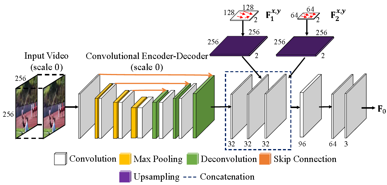
\hat{Y}_0=\mathcal{T}(X,F_0)=\mathcal{T}(X,\mathcal{H}(X;\Theta,F_N,\ldots,F_1))
Refinement
Multi-scale Flow Fusion
Extension
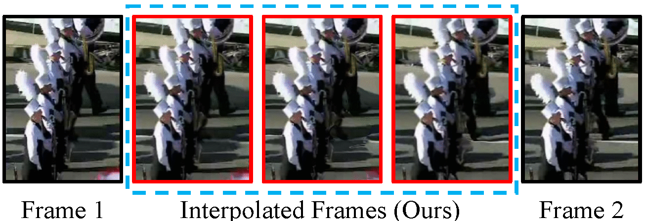
Multi-step Prediction
Predict D frames given current L frames
\hat{Y} \in \mathbb{R}^{H \times W}\Rightarrow \hat{Y} \in \mathbb{R}^{H \times W \times D}
\hat{Y}(x,y)\Rightarrow \hat{Y}(x,y,t)
Smaller learning rate: 0.00005
Experiment
Compete with the State-of-the-art
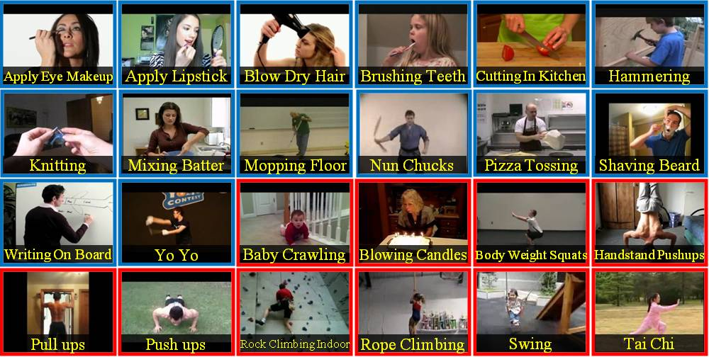
Training set: UCF-101 Train, 240k triplets
Test set: UCF-101 Test, THUMOS-15
Competing methods (state-of-the-art)
- EpicFlow + algorithm from Middlebury interpolation benchmark
- BeyondMSE(with little tweaks)
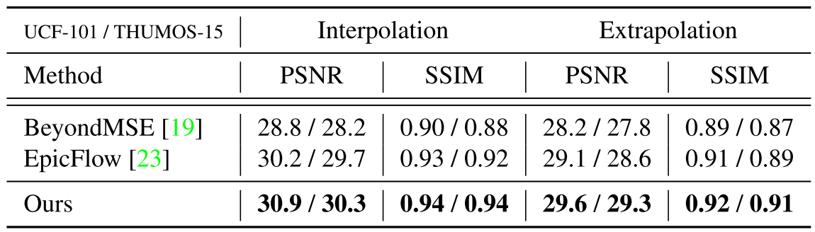
Experiment
Compete with the State-of-the-art
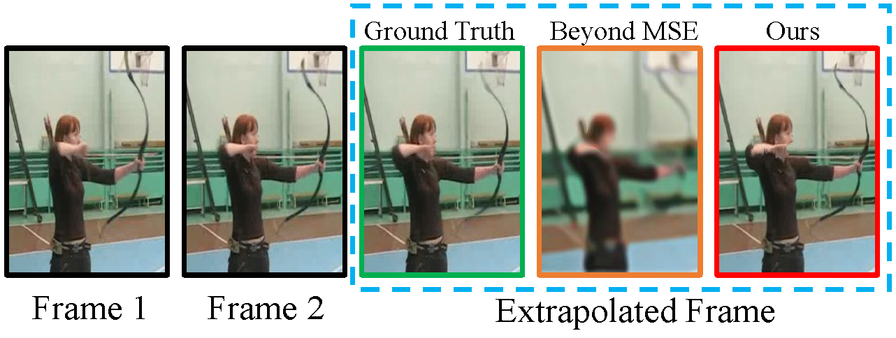
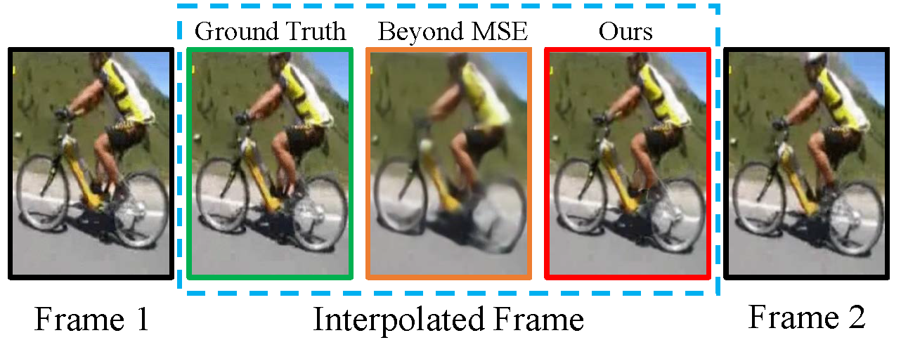
Experiment
Compete with the State-of-the-art
Interpolation
Extrapolation
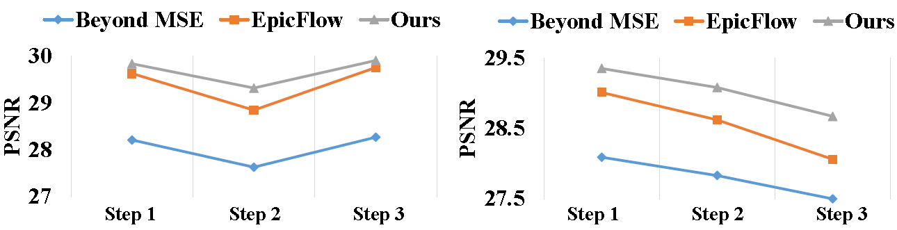
Multi-step comparisons
Experiment
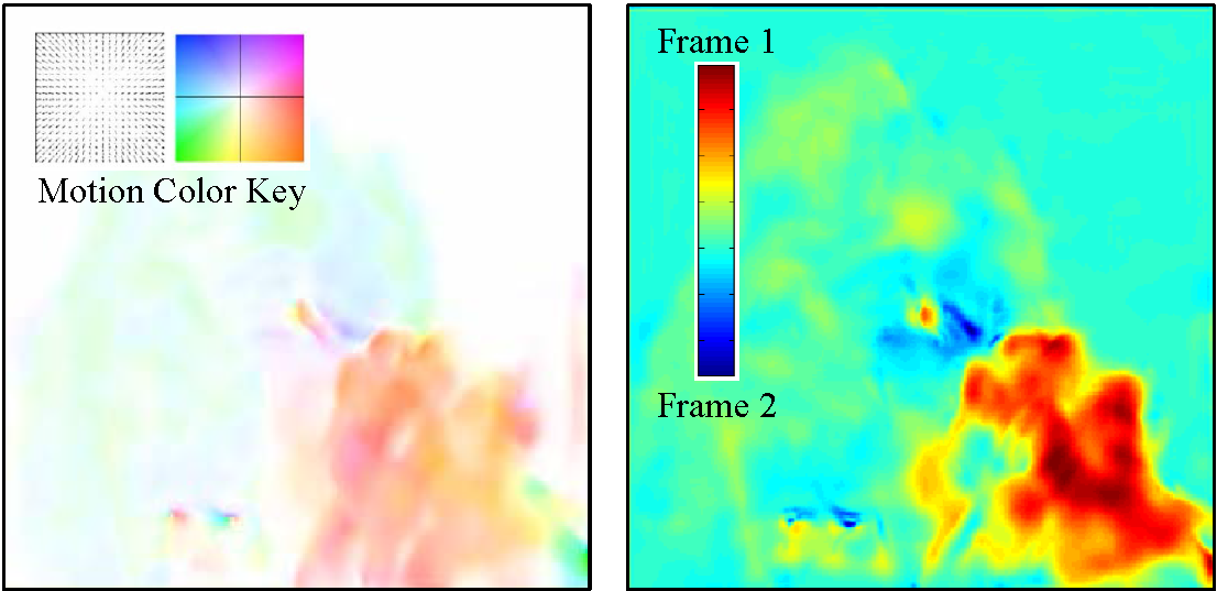
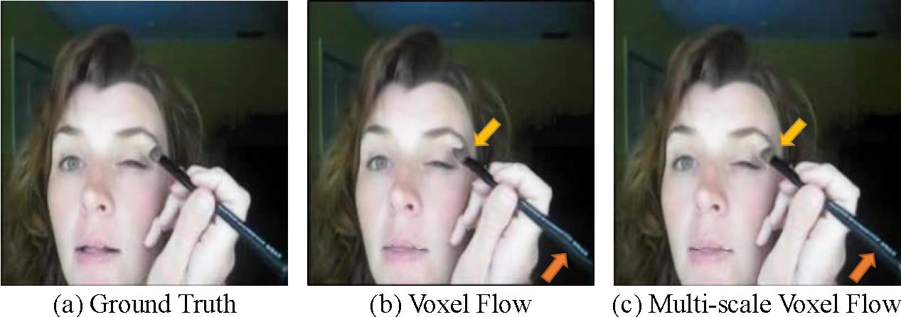
Effectiveness of Multi-scale Voxel Flow
Appearance
Motion
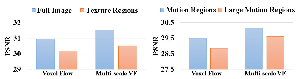
UCF-101 test set
Experiment
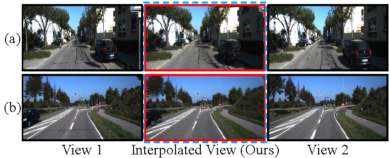
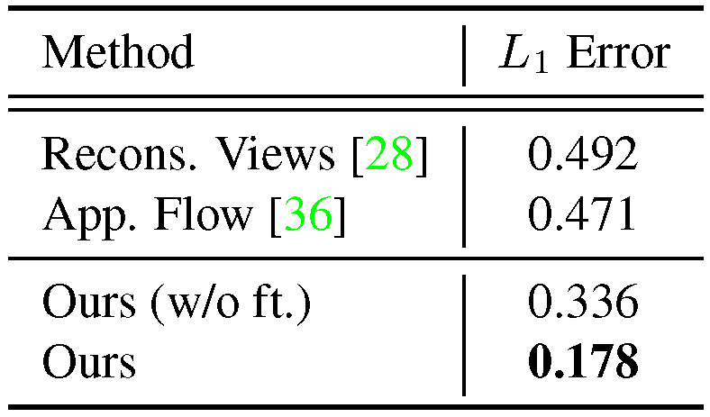
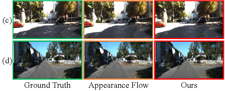
Generalization to View Synthesis
Evaluate KTTI odometry dataset
Experiment
Generalization to View Synthesis
Experiment
Frame Synthesis as Self-Supervision
Video frame synthesis can serve as a self-supervision task for representation learning( )
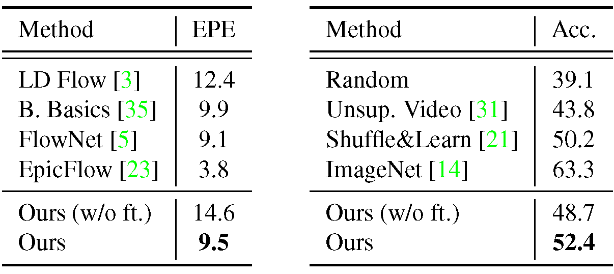
Flow estimation
(endpoint error)
Action recognition
\mathcal{H}\left( X;\Theta \right)
Experiment
Application
Produce slow-motion effects on HD videos(1080x720, 30fps)
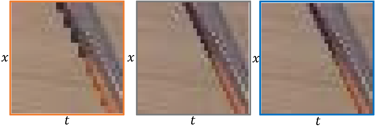
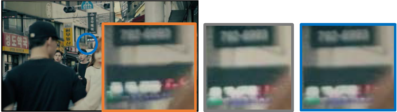
- Visual Comparison
- User Study
EpicFlow serve as a strong baseline
Experiment
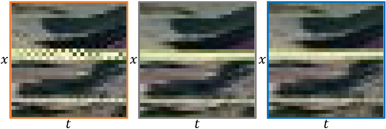
Application-Visual Comparison
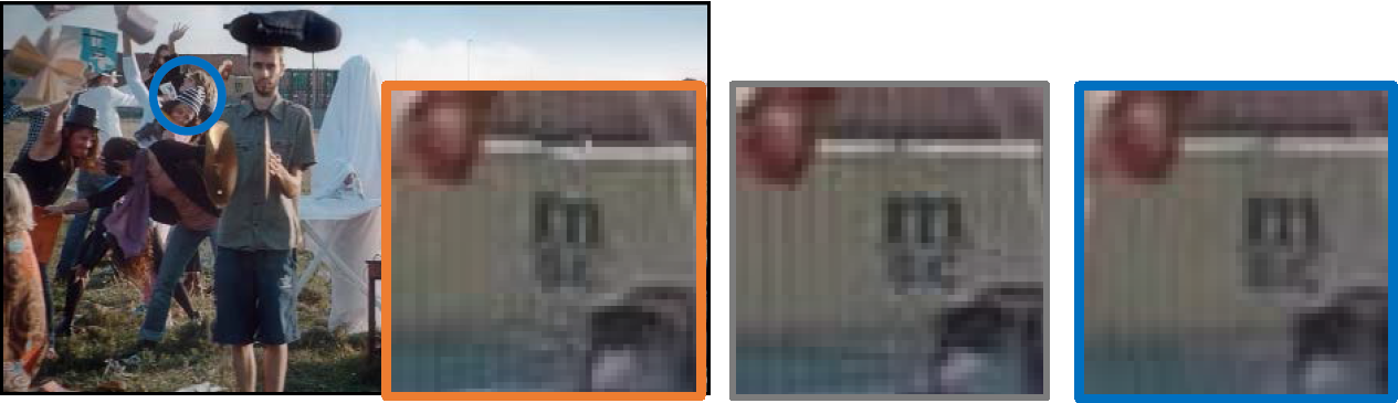
EpicFlow
Ground Truth
DVF
Experiment
Application-Visual Comparison
EpicFlow
Ground Truth
DVF
Experiment
Application-User Study
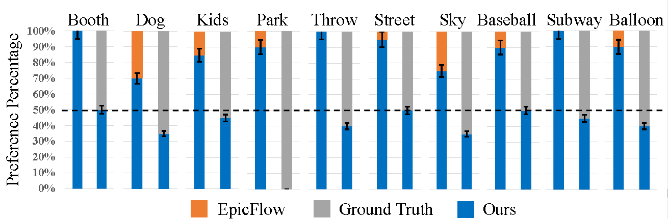
20 subjects were enrolled
For the null hypothesis:
- "EpicFlow is better than our method"
p-value < 0.00001 - "DVF is better than ground truth"
p-value < 0.838193
Experiment
Demo Video
Summary
- End-to-end deep network
- Copy pixels from existing video frames, rather than hallucinate them from scratch
- Improves upon both optical flow and recent CNN techniques
Future Work
- Combine flow layers with pure synthesis layers
⇒ predict pixels that cannot be copied from other video frames - Use the desired temporal step as an input
- Compress the network, and run on mobile devices
Video Frame Synthesis using Deep Voxel Flow
By Maeglin Liao


