\text{Tomancak Lab, Group Meeting}
\text{Dec 15, 2020}
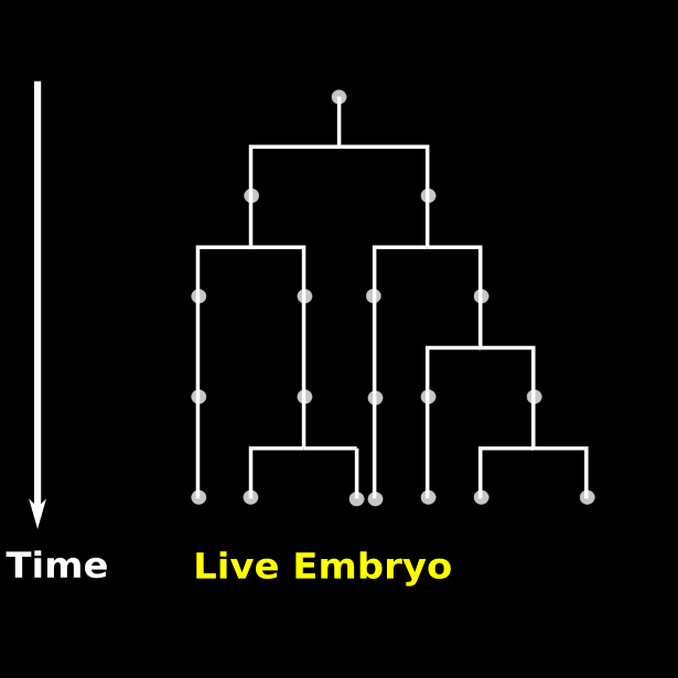
\text{Early development of an organism}
\text{Nuclei}
\text{Membrane}
\text{Light sheet Imaging}
\text{Time-lapse recording of Embryo 1}
\text{Early development of an organism}
\text{Nuclei}
\text{Membrane}
\text{Light sheet Imaging}
\text{Time-lapse recording of Embryo 1}
\text{Confocal Imaging}
\text{Embryo 2}
\text{Embryo ...}
\text{Embryo N}
\text{Nuclei}
\text{Gene}
\text{Membrane}
\text{Our model organism}
\text{\textit{Platynereis dumerillii}}
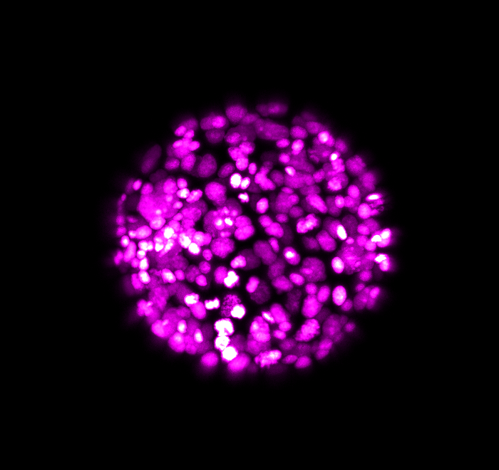
\text{Light Sheet Imaging of Live Embryo}
\text{Confocal Images of specimens}
\text{Adult worm}
\text{Embryo @ 16 hpf*}
\text{hpf*: hours post fertilization}
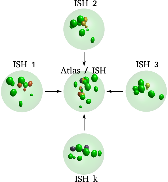
\text{at 16 hpf using ISH*}
\text{ISH*: \textit{in situ} hybridization}

\text{Adult worm}
\text{Our problem statement}
\text{Our problem statement}
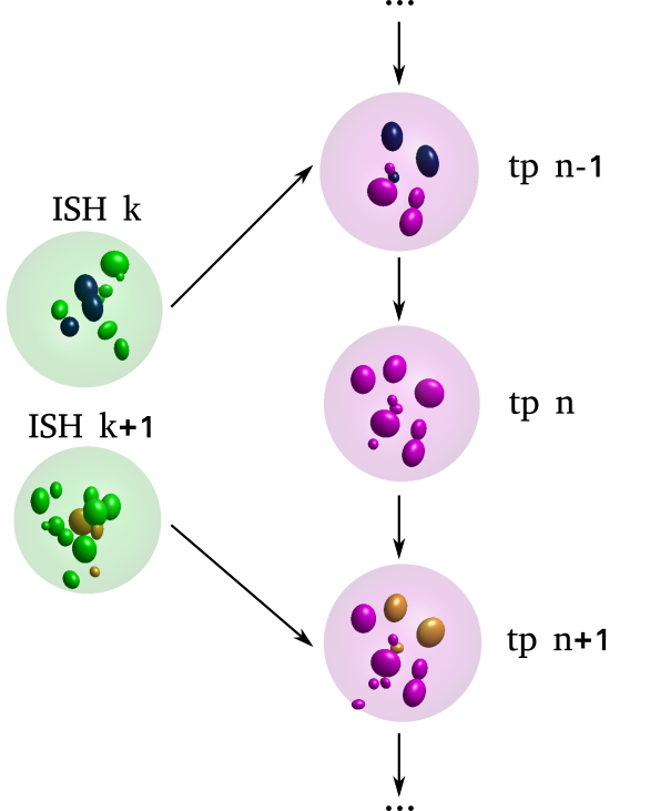
\text{Intramodal Registration}
\text{Intermodal Registration}
\text{* tp: time point}
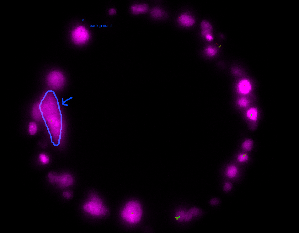
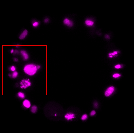
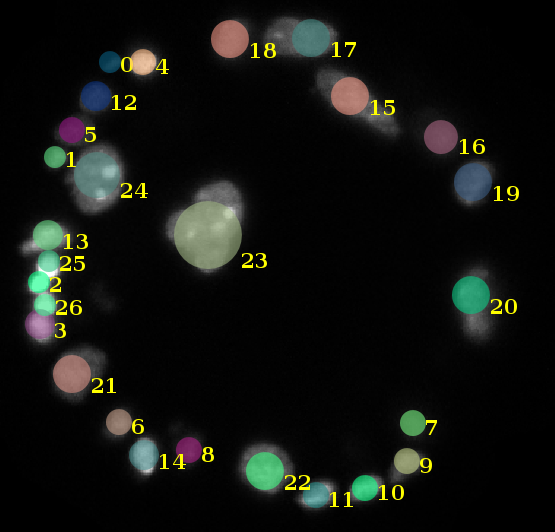
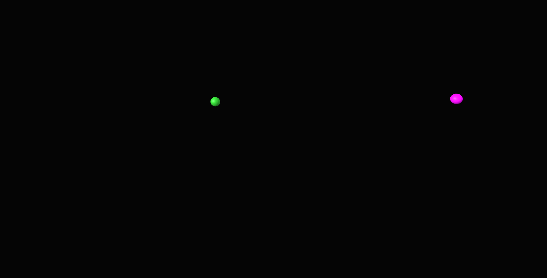
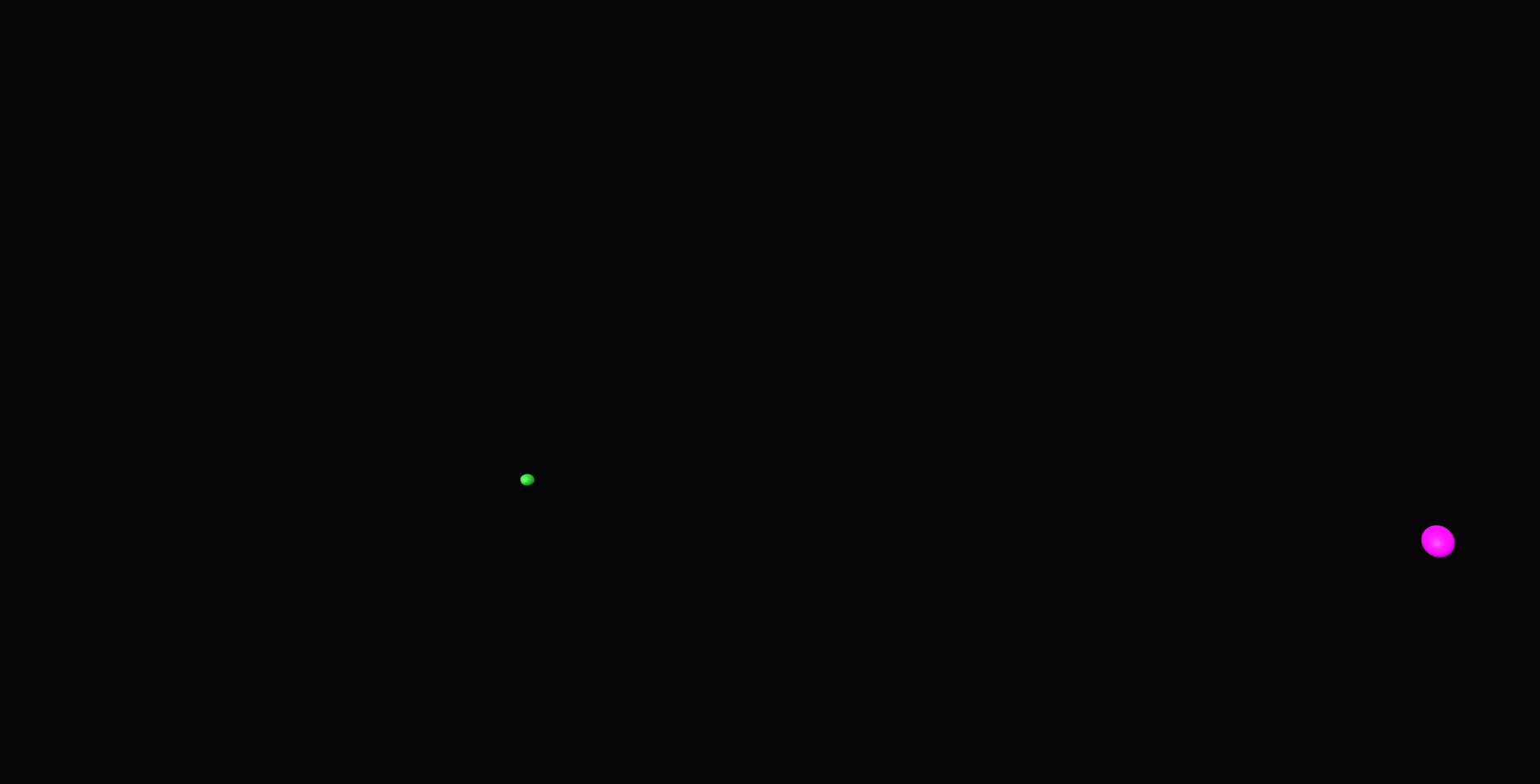
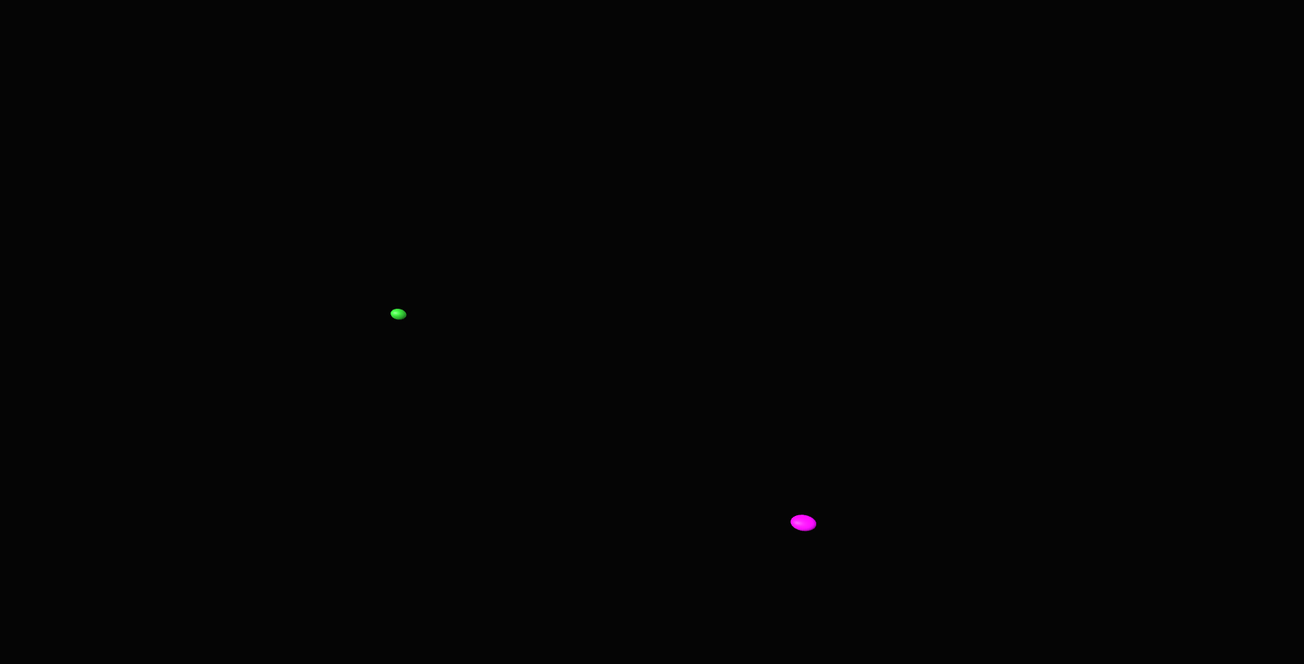
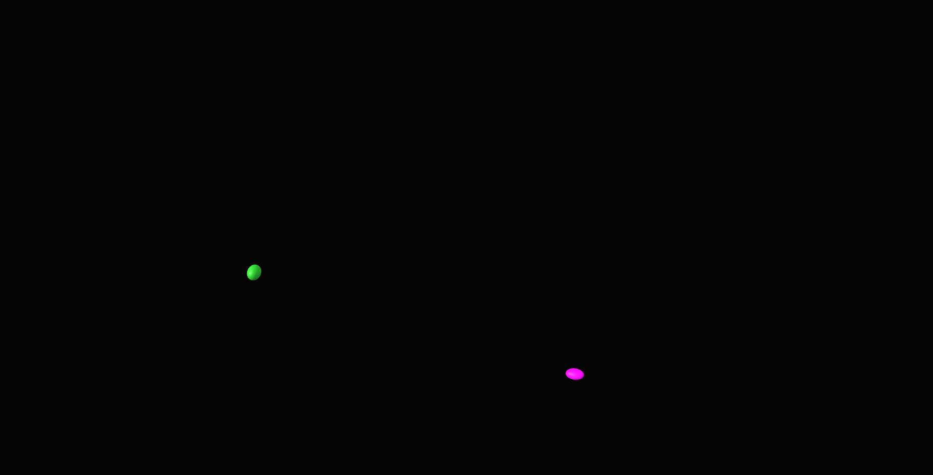
\text{Challenges in identifying nuclei correspondence}

\text{Live Embryo:}
\text{Nuclei}
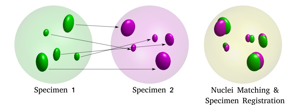
\text{Cell nuclei positions were fitted to an}
\text{ellipsoid}

situ
\text{Nuclei}
\text{Cell nuclei positions were fitted to an}
\text{ellipsoid}
In-
\text{specimen:}
\text{How to identify cell-to-cell correspondences?}
\text{Morphology}
\text{Appearance}
\text{Geometric Arrangement}

\text{Use distinctively shaped nuclei to align and match}
\text{Use neighborhood as a feature to identify corrsponding nuclei}
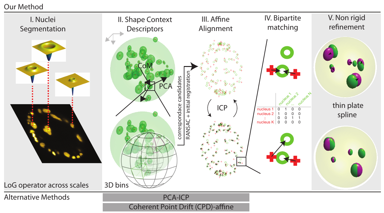
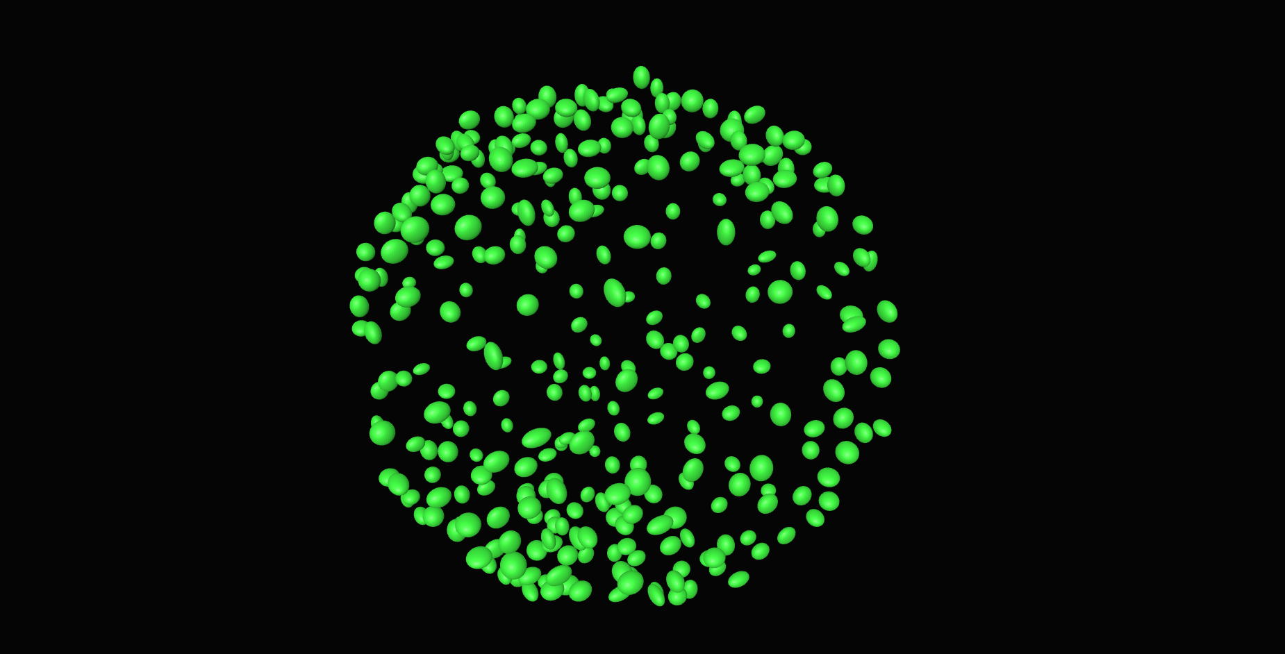
\text{Our approach}
\sigma=6
\sigma=7
\sigma=5
\sigma=8
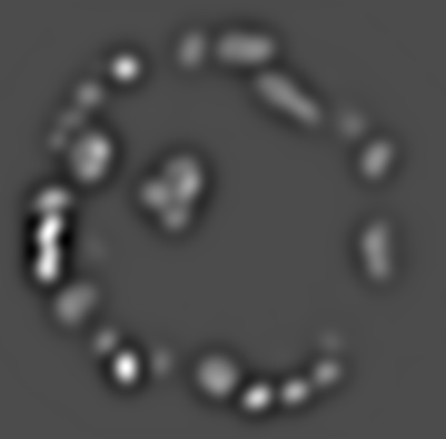
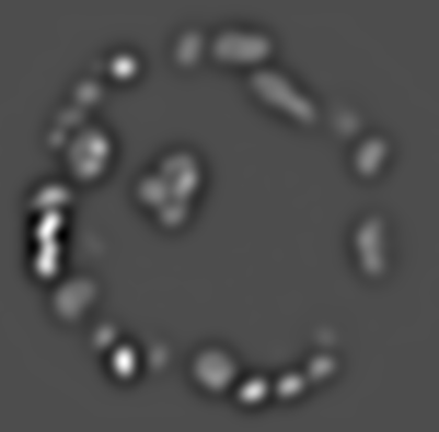
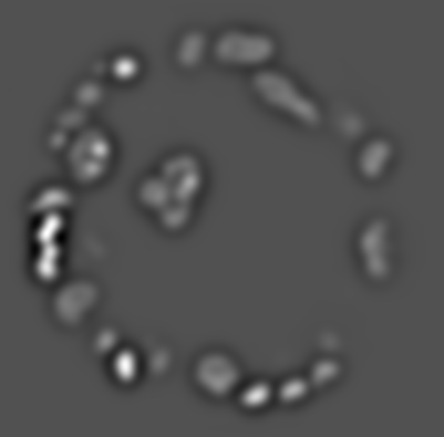
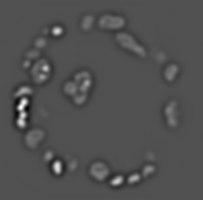
\text{1. Evaluate }\nabla^{2} G_{\sigma} \circledast \mathbf{I}
\text{Our approach}
\sigma=6
\sigma=7
\sigma=5
\sigma=8
\text{1. Evaluate }\nabla^{2} G_{\sigma} \circledast \mathbf{I}
\text{2. Find local minima }
\text{in x, y, z, $\sigma$ space}
\text{Our approach}
\text{Our approach}
\text{Belongie et al.``Shape matching and object recognition using shape contexts"}
\text{IEEE Transactions on Pattern Analysis and Machine Intelligence, 2002}
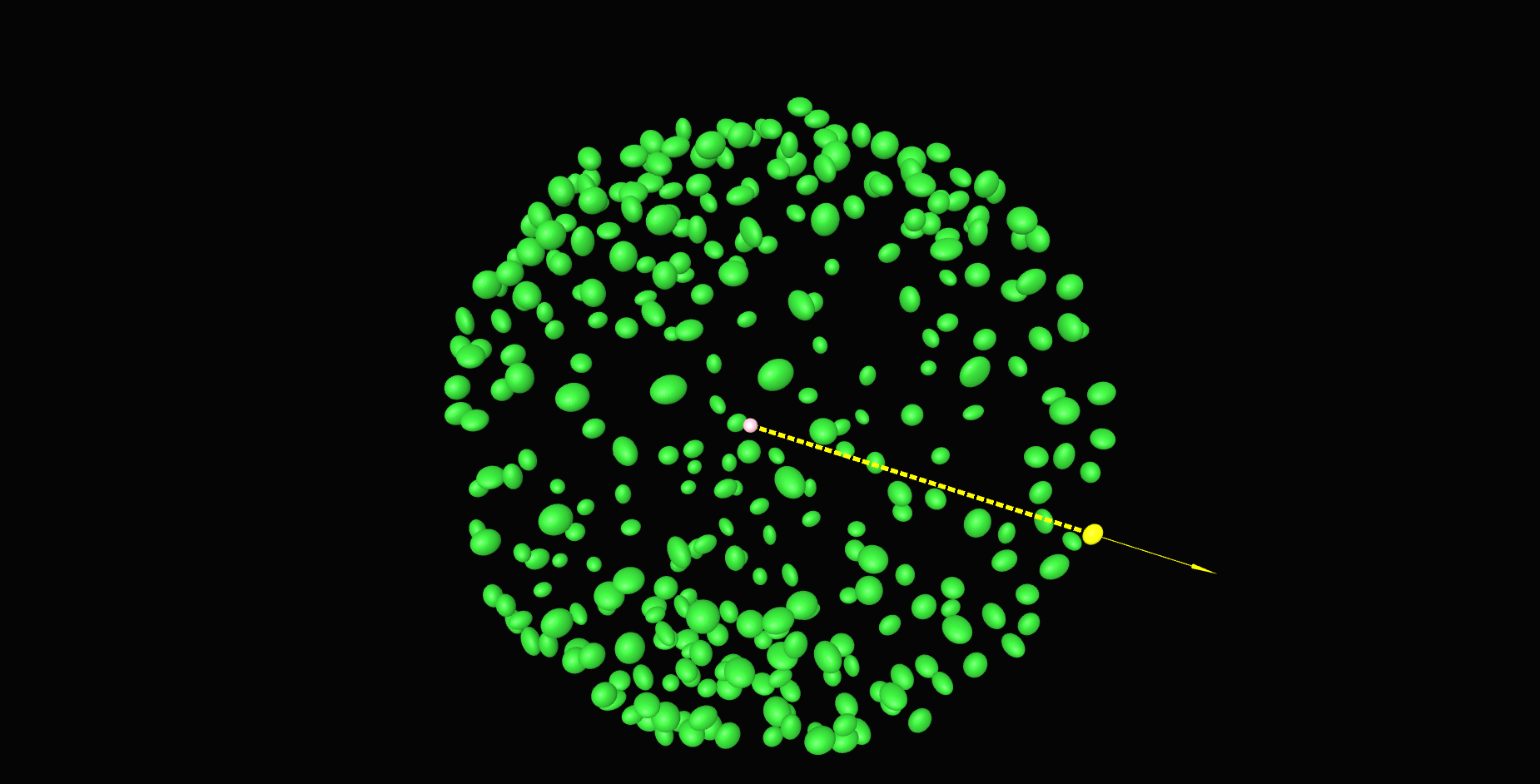
\text{Z'}
\text{Our approach}
\text{Y'}
\text{Z'}
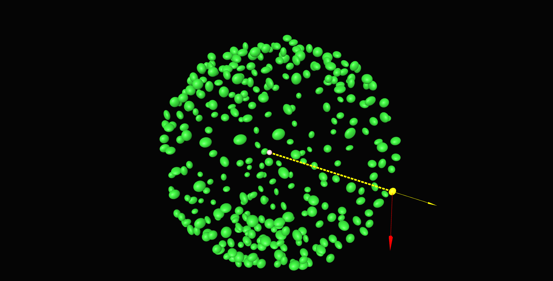
\text{Our approach}

\text{Z'}
\text{Y'}
\text{X'}
\text{Our approach}

\text{Our approach}


3
11
15
6
12
4
0
9
0
0
22
3
5
17
11
19
\text{Bins: }
\text{1}
\text{2}
\text{3}
\text{4}
\text{...}
\text{...}
\text{K}
6
6
6
0
0
0
2
2
4
4
4
4
20
18
14
13
16
16
9
19
\text{Nucleus 1 @ (12, 34, 89)}
\text{Nucleus 2 @ (26, 49, 92)}
\text{Nucleus 3 @ (68, 93, 21)}
\text{Nucleus 4 @ (81, 32, 15)}
\text{Nucleus ... @ (..., ..., ...)}
\text{Our approach}
0.03
0.1
0.1
0.06
0.1
0.01
0
0.03
0
0
0.2
0.01
0.02
0.2
0.1
0.2
\text{Bins: }
\text{1}
\text{2}
\text{3}
\text{4}
\text{...}
\text{...}
\text{K}
0.1
0.02
0.02
0
0
0
0.01
0.01
0.01
0.01
0.01
0.01
0.2
0.2
0.1
0.1
0.2
0.2
0.03
0.2
\text{Nucleus 1 @ (12, 34, 89)}
\text{Nucleus 2 @ (26, 49, 92)}
\text{Nucleus 3 @ (68, 93, 21)}
\text{Nucleus 4 @ (81, 32, 15)}
\text{Nucleus ... @ (..., ..., ...)}
\sum^{k=K}_{k=1} h(k) =1
\text{Our approach}
\text{...}


C_{ij} := C(p_{i}, q_{j})
\text{1}
\text{1'}
\text{2}
\text{2'}
\text{3}
\text{3'}
\text{4}
\text{4'}
\text{2}
\text{...}
p_{1}
p_{2}
p_{3}
p_{4}
p_{...}
p_{M}
q_{1}
q_{2}
q_{3}
q_{4}
q_{M}
q_{...}
= \frac{1}{2} \sum_{k=1}^{K} \frac{(h_{i}(k) -h_{j}(k))^{2}}{h_{i}(k) + h_{j}(k)}
\text{0.24}
\text{0.19}
\text{0.21}
\text{0.12}
\text{0.15}
\text{0.18}
\text{0.06}
\text{0.23}
\text{0.16}
\text{0.07}
\text{0.16}
\text{0.13}
\text{0.29}
\text{0.15}
\text{0.28}
\text{0.20}
\text{0.11}
\text{0.14}
\text{0.18}
\text{0.13}
\text{0.24}
\text{0.26}
\text{0.12}
\text{0.09}
\text{0.14}
\text{0.17}
\text{0.23}
\text{0.26}
\text{0.19}
\text{0.22}
\text{0.14}
\text{0.16}
\text{0.23}
\text{0.21}
\text{0.11}
\text{0.09}
\text{Our approach}
\textit{Apply RANSAC to estimate}
\textit{coarse transform using inliers}
\begin{bmatrix}
1^{'}_{x} & 2^{'}_{x} & 3^{'}_{x} & 4^{'}_{x}\\
1^{'}_{y} & 2^{'}_{y} & 3^{'}_{y} & 4^{'}_{y}\\
1^{'}_{z} & 2^{'}_{z} & 3^{'}_{z} & 4^{'}_{z}\\
\end{bmatrix}=
A \times
\begin{bmatrix}
1_{x} & 2_{x} & 3_{x} & 4_{x}\\
1_{y} & 2_{y} & 3_{y} & 4_{y}\\
1_{z} & 2_{z} & 3_{z} & 4_{z}\\
\end{bmatrix}
\text{Sample 4 pairs of correspondences}
\text{Our approach}
\text{``Random sample consensus: A paradigm for model fitting with applications to image analysis and automated cartography.''}
\text{Fischer and Bolles, Communications of the ACM (1981)}
\text{Count Inliers}
\textit{Apply RANSAC to estimate}
\textit{coarse transform using inliers}
\begin{bmatrix}
1^{'}_{x} & 2^{'}_{x} & 3^{'}_{x} & 4^{'}_{x}\\
1^{'}_{y} & 2^{'}_{y} & 3^{'}_{y} & 4^{'}_{y}\\
1^{'}_{z} & 2^{'}_{z} & 3^{'}_{z} & 4^{'}_{z}\\
\end{bmatrix}=
A \times
\begin{bmatrix}
1_{x} & 2_{x} & 3_{x} & 4_{x}\\
1_{y} & 2_{y} & 3_{y} & 4_{y}\\
1_{z} & 2_{z} & 3_{z} & 4_{z}\\
\end{bmatrix}
\text{Sample 4 pairs of correspondences}
\text{Our approach}
\text{Repeat}
\text{Count Inliers}
\textit{Apply RANSAC to estimate}
\textit{coarse transform using inliers}
\begin{bmatrix}
1^{'}_{x} & 2^{'}_{x} & 3^{'}_{x} & 4^{'}_{x}\\
1^{'}_{y} & 2^{'}_{y} & 3^{'}_{y} & 4^{'}_{y}\\
1^{'}_{z} & 2^{'}_{z} & 3^{'}_{z} & 4^{'}_{z}\\
\end{bmatrix}=
A \times
\begin{bmatrix}
1_{x} & 2_{x} & 3_{x} & 4_{x}\\
1_{y} & 2_{y} & 3_{y} & 4_{y}\\
1_{z} & 2_{z} & 3_{z} & 4_{z}\\
\end{bmatrix}
\text{Sample 4 pairs of correspondences}
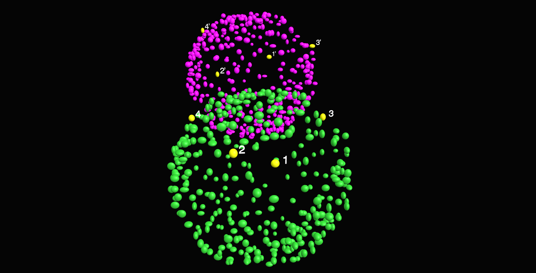
\text{Our approach}

\text{...}
\text{...}
p^{*}_{1}
p^{*}_{2}
p^{*}_{3}
p^{*}_{4}
p^{*}_{...}
p^{*}_{M}
q_{1}
q_{2}
q_{3}
q_{4}
q_{N}
q_{...}
\text{10.1}
\text{2.6}
\text{11.3}
\text{89.7}
\text{14.2}
\text{90.8}
\text{64.2}
\text{23.5}
\text{16.9}
\text{70.8}
\text{16.7}
\text{32.4}
\text{9.7}
\text{15.4}
\text{28.3}
\text{20.1}
\text{11.6}
\text{14.9}
\text{18.1}
\text{3.7}
\text{24.1}
\text{36.4}
\text{12.2}
\text{9.5}
\text{14.2}
\text{17.5}
\text{23.45}
\text{6.7}
\text{19.9}
\text{22.1}
\text{14.8}
\text{16.4}
\text{63.7}
\text{21.5}
\text{81.1}
\text{9.6}
C_{ij} := C(p^{*}_{i}, q_{j})
= \sqrt{\left( p^{*}_{i,x} -q_{j,x} \right)^{2} + \left( p^{*}_{i,y} -q_{j,y} \right)^{2} + \left( p^{*}_{i,z} -q_{j,z} \right)^{2}}
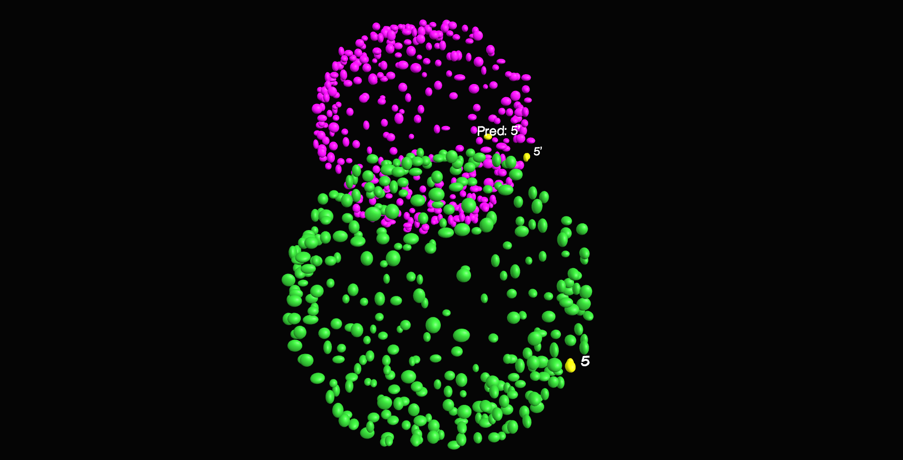
\text{1}
\text{5'}
\text{1'. 4'}
\text{3}
\text{2'}
\text{4}
\text{6'}
\text{2}
\text{3'}
\text{Find Nearest Neighbor Correspondences}
\textit{Apply ICP to obtain a tighter fit}
\text{Our approach}
\textit{Apply ICP to obtain a tighter fit}
\text{Find Nearest Neighbor Correspondences}
\text{Estimate Affine Transform}
\begin{bmatrix}
1^{'}_{x} & 2^{'}_{x} & \ldots & M^{'}_{x}\\
1^{'}_{y} & 2^{'}_{y} & \ldots & M^{'}_{y}\\
1^{'}_{z} & 2^{'}_{z} & \ldots & M^{'}_{z}\\
\end{bmatrix}=
A \times
\begin{bmatrix}
1_{x} & 2_{x} & \ldots & M_{x}\\
1_{y} & 2_{y} &\ldots & M_{y}\\
1_{z} & 2_{z} & \ldots & M_{z}\\
\end{bmatrix}
\text{Our approach}
\textit{Apply ICP to obtain a tighter fit}
\text{Find Nearest Neighbor Correspondences}
\text{Estimate Affine Transform}
\text{Repeat upto Convergence}
\text{Our approach}
\text{...}
\text{...}
p^{*}_{1}
p^{*}_{2}
p^{*}_{3}
p^{*}_{4}
p^{*}_{...}
p^{*}_{M}
q_{2}
q_{3}
q_{4}
q_{N}
q_{...}
\text{4.1}
\text{2.6}
\text{11.3}
\text{89.7}
\text{14.2}
\text{90.8}
\text{64.2}
\text{7.8}
\text{16.9}
\text{70.8}
\text{16.7}
\text{32.4}
\text{9.7}
\text{15.4}
\text{8.3}
\text{20.1}
\text{11.6}
\text{14.9}
\text{18.1}
\text{3.7}
\text{24.1}
\text{36.4}
\text{12.2}
\text{9.5}
\text{14.2}
\text{17.5}
\text{23.45}
\text{6.7}
\text{19.9}
\text{22.1}
\text{14.8}
\text{16.4}
\text{63.7}
\text{21.5}
\text{81.1}
\text{9.6}
q_{1}
\textit{to obtain one-to-one matching }
C_{ij} := C(p^{*}_{i}, q_{j})
= \sqrt{\left( p^{*}_{i,x} -q_{j,x} \right)^{2} + \left( p^{*}_{i,y} -q_{j,y} \right)^{2} + \left( p^{*}_{i,z} -q_{j,z} \right)^{2}}
\hat{X}= \underset{X}{\text{arg min}} \sum_{i=1}^{M} \sum_{j=1}^{N} C_{ij} X_{ij}
\text{ where } X_{ij} \in \{0, 1\}
\text{ s.t.} \sum_{k=1}^{k=M} X_{ik} = 1
\sum_{k=1}^{k=N} X_{kj} \leq 1
\text{Our approach - at the time of $BIC^{*}$}
\textit{Apply Hungarian Algorithm}
^{*}\text{BioImage Computing, ECCV 2020}

\text{Intra-modal}
\text{Inter-modal}
\text{registration}
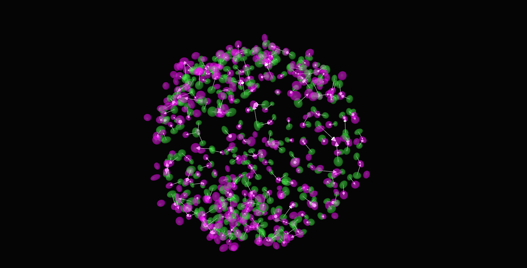
\text{Before}
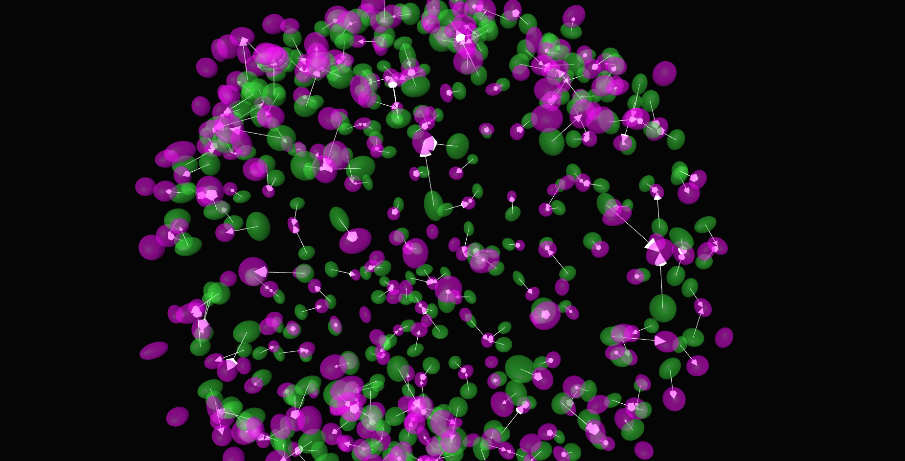
\text{Results (}
\text{Intra-modal}
\text{Inter-modal}
\text{registration)}
\text{\textit{after}}
\text{Results (}
\text{registration)}
\text{\textit{after}}
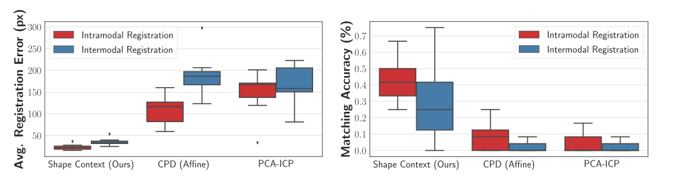
\text{Conclusions - at the time of BIC}
\text{Intra-modal}
\text{Inter-modal}
\text{We demonstrated a pipeline for registering volumetric images of embryos}
\text{by establishing correspondences between cells}
\text{Our approach produces lower average registration error than baselines on real data}
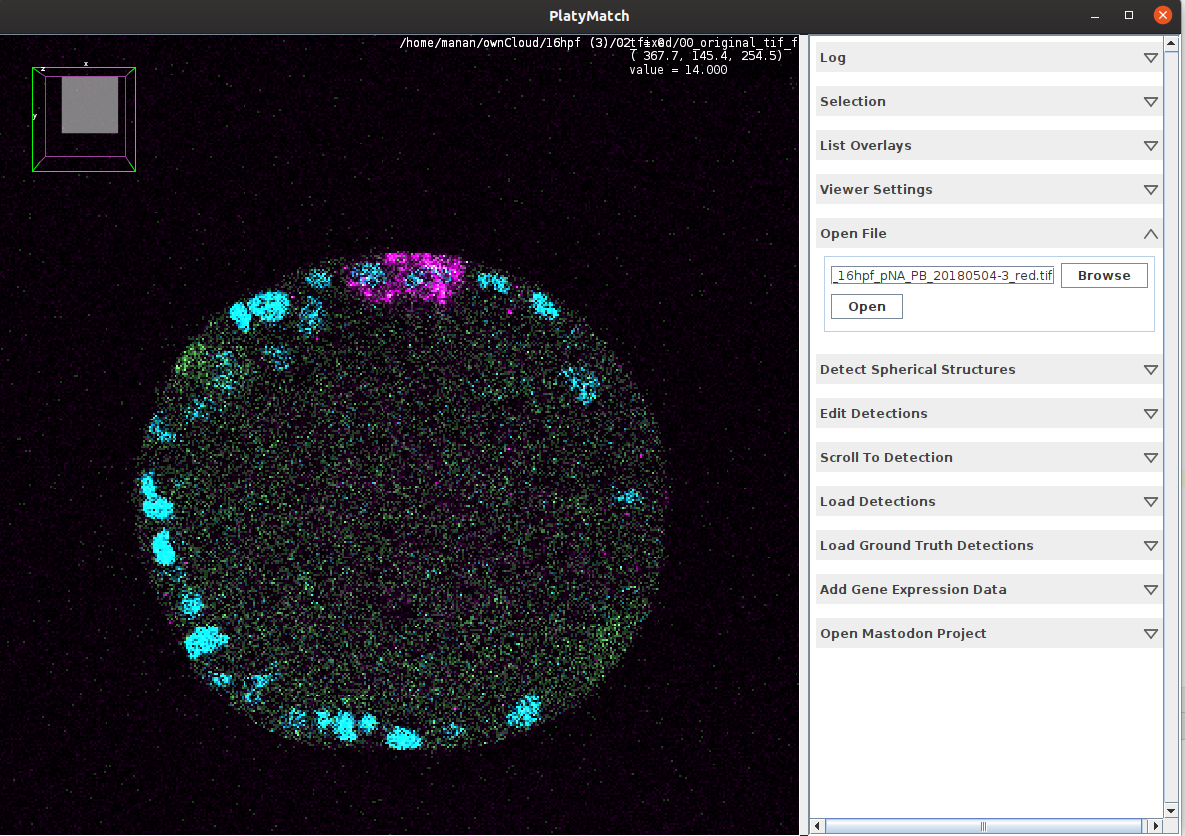
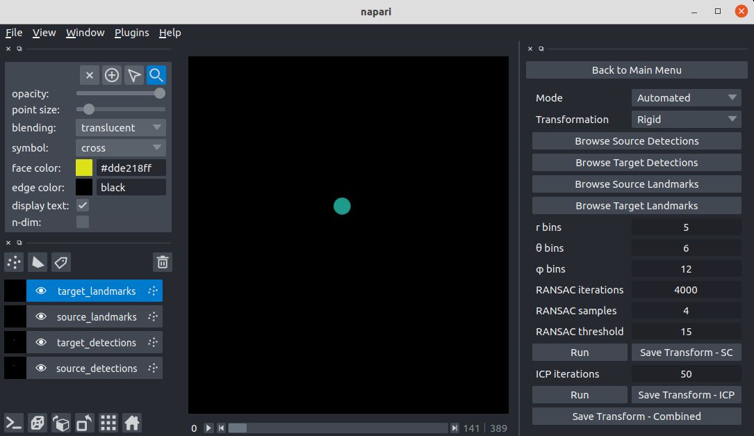
\text{We developed a FIJI \& Napari plugin for easier useability }
\text{BUT there is error in matching nuclei}
\text{Modify Last Step - Benefit from Tracking GT data}
\text{Inter-modal}
\text{t = T }
\text{t = T + K}
\ldots
\ldots
\text{t = T - K}
C^{T-K}
C^{T}
C^{T+K}
\ldots
\ldots
\text{Use $C^{T-K}$, \ldots, $C^{T}$, \ldots, $C^{T+K}$ to determine the best $X$ that respects the tracking!}
\text{Instance Segmentation}
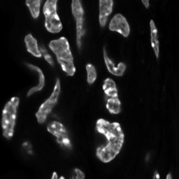
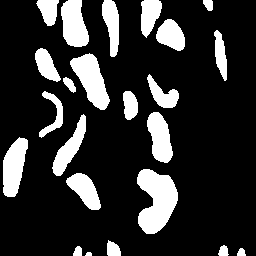
\text{Instance Segmentation}
\text{Unique Segmentation of Each Nucleus/Cell}
1
2
3
4
5
6
7
8
9
10
11
12
13
14
15
16
17
\text{EmbedSeg 2D$^{*}$}
1
2
3
4
5
6
7
8
9
10
11
12
13
14
15
16
17
\text{Pixels belonging to one object should be embedded together}
\text{Pixels belonging to different objects should be embedded separately }
*\text{Under review at ISBI, 2021}
\text{``Instance Segmentation by Jointly Optimizing Spatial Embeddings and Clustering Bandwidth''}
\text{Neven et al, CVPR, June 2019}
\text{Results}
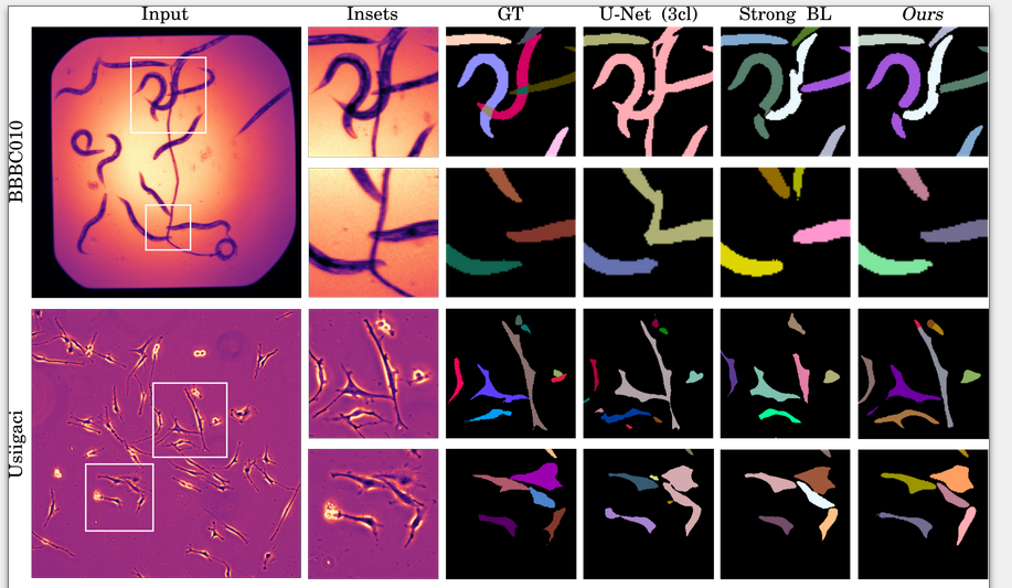
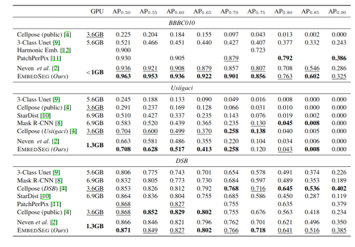
\text{Why Another Method?}
\text{CellPose addresses 3D segmentation through a proxy approach}
\text{StarDist3D consumes large GPU memory and has blocky appearance}


\text{Why Another Method?}
\text{CellPose addresses 3D segmentation through a proxy approach}
\text{StarDist3D consumes large GPU memory and has blocky appearance}

\text{Annotating Platynereis Data}


\text{Future directions}
\text{Predict instance shapes on both live embryo and in-situ images at 16, 20 and 24 hours}
\text{Use morphology information in addition to geometric arrangement for matching}
\text{Embryo at 16 hpf}
\text{Nuclei}
\text{Pax3/7}
\text{Embryo at 20 hpf}
\text{Nuclei}
\text{Pax3/7}


\text{See if the network can learn a neighborhood descriptor on its own}
\text{Thank You for Listening!}

Group Meeting, Tomancak Lab
By Manan Lalit
Group Meeting, Tomancak Lab
Dec 15, 2020

