Interactive Intro
LSTM
Text
Text
Introduction to LSTM

Interactive Intro
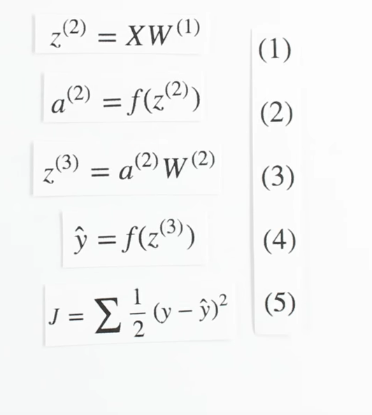
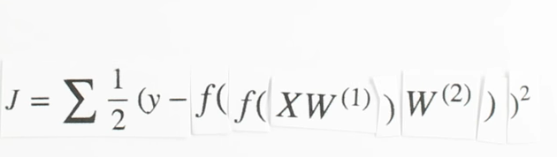
Neural Networks
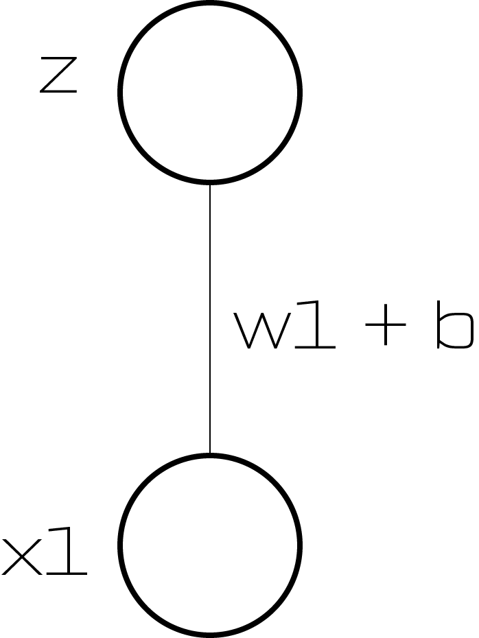
Neuron

Chapter 1 | Recurrent NN
Interactive Intro
Neural Networks
Neuron
Chapter 1 | Recurrent NN
Chapter | Recurrent NN
Chapter | LSTM
Use cases
Chapter | LSTM
Use cases
Chapter | LSTM
Interactive Intro
Neural Networks
Chapter 1 | Recurrent NN
Interactive Intro
Neural Networks
Chapter 1 | Recurrent NN
Chapter | Reccurent NN

Chapter | Reccurent NN
Chapter | LSTM
Chapter | LSTM
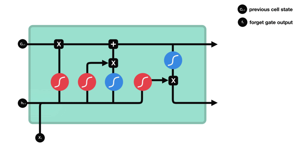
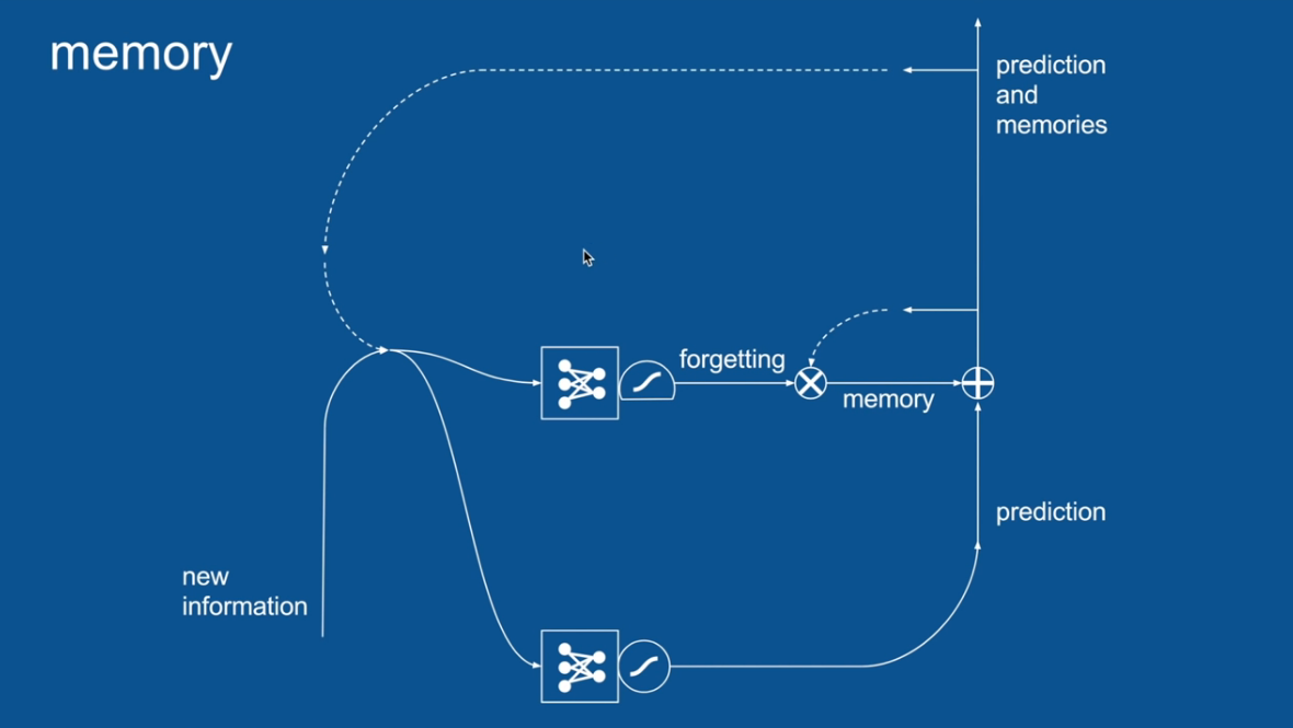
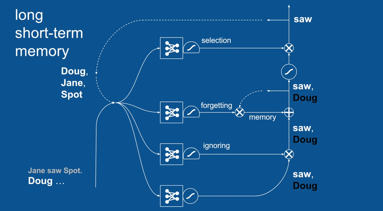
Some Forgotten Some Remembered
Chapter | LSTM
Entire Neural Net Dedicated to
forgetting/Remembering
Chapter | LSTM
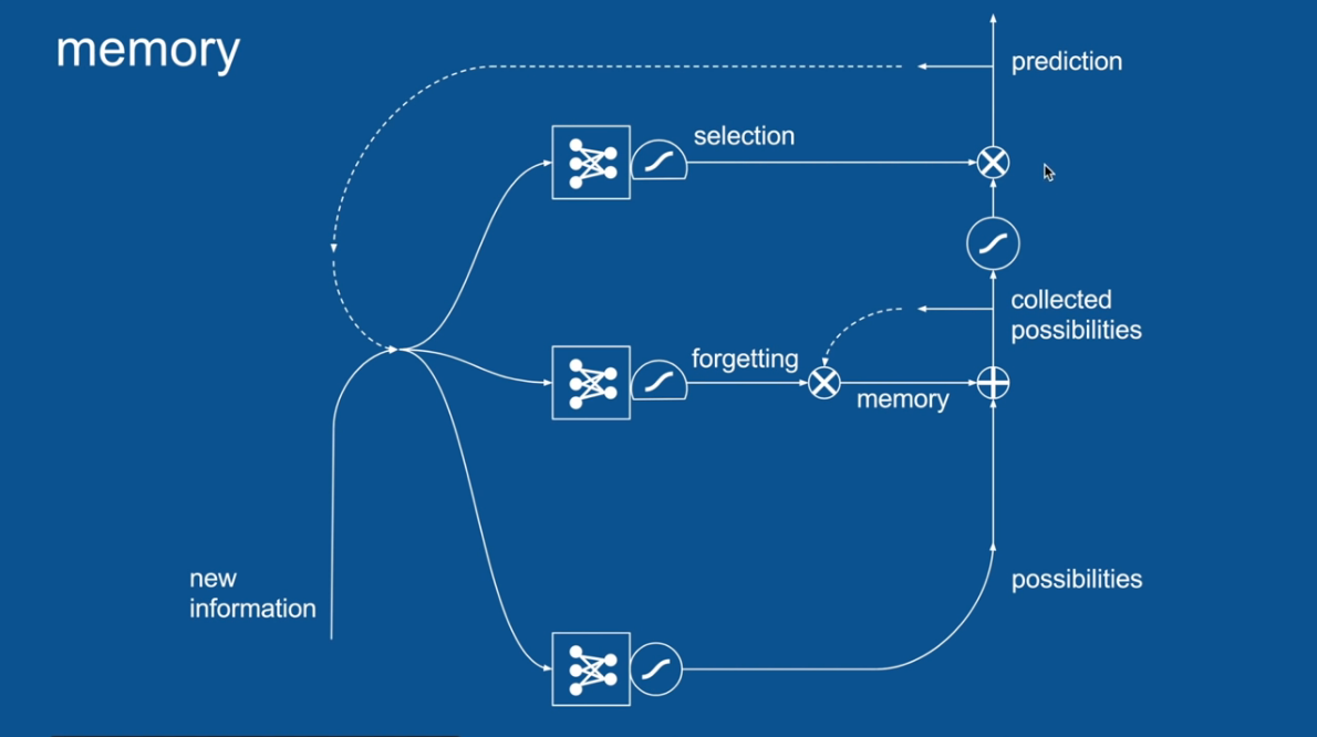
Chapter | LSTM
A selection that has its own neural network
to filter out the memory used in the prediction
Chapter | LSTM
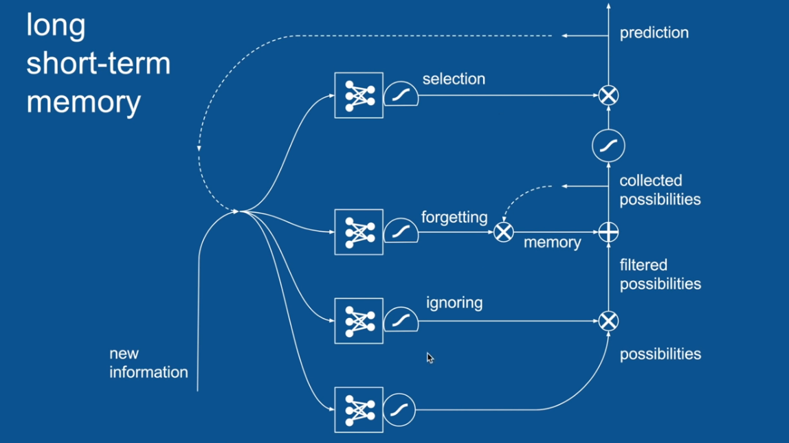
Chapter | LSTM
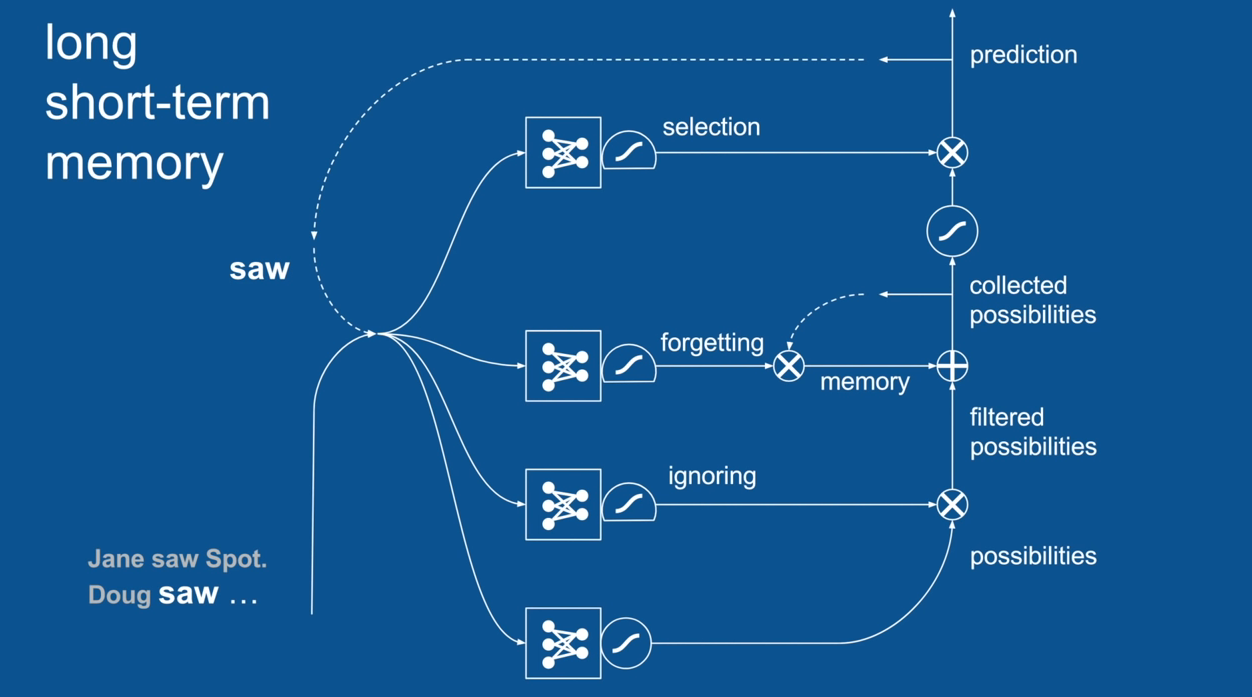
Ignore Irrelevance
Chapter | LSTM
Ignore Irrelevance
Chapter | LSTM
Ignore Irrelevance
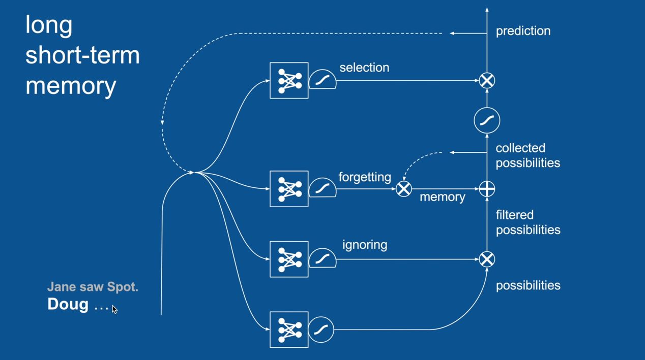
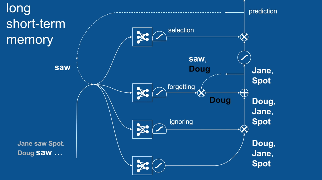
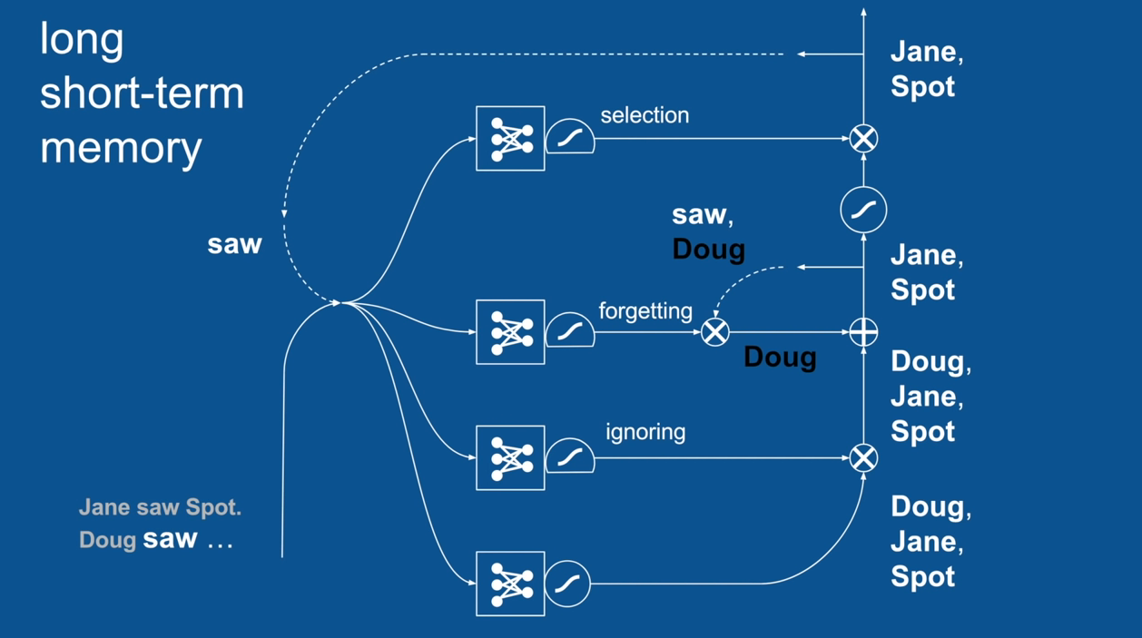
Practical Example: Sentence Prediction
Jane saw Spot. <PREDICTION>
Chapter | LSTM
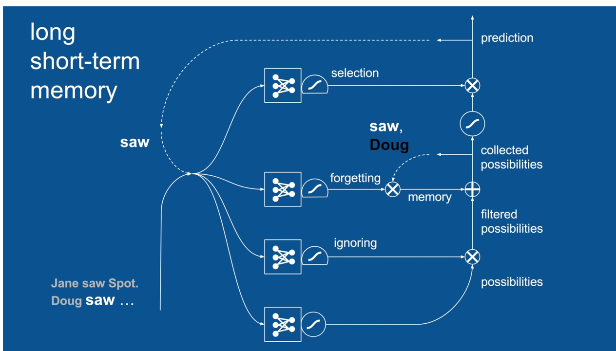
Ignore Irrelevance
Practical Example: Sentence Prediction
Chapter | LSTM
Ignore Irrelevance
Practical Example: Sentence Prediction
Chapter | LSTM
Ignore Irrelevance
Practical Example: Sentence Prediction
Jane saw Spot. Doug <PREDICTION>
Chapter | LSTM
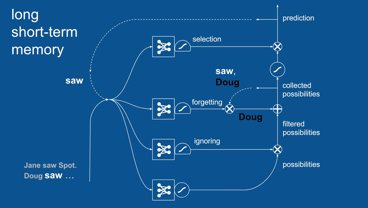
Ignore Irrelevance
Practical Example: Sentence Prediction
Chapter | LSTM
Ignore Irrelevance
Practical Example: Sentence Prediction
Chapter | LSTM
Ignore Irrelevance
Practical Example: Sentence Prediction
Chapter | LSTM
Ignore Irrelevance
Practical Example: Sentence Prediction
Chapter | LSTM
Ignore Irrelevance
Practical Example: Sentence Prediction
Chapter | LSTM
Ignore Irrelevance
Practical Example: Sentence Prediction
Chapter | LSTM
Ignore Irrelevance
Practical Example: Sentence Prediction
Chapter | LSTM
Ignore Irrelevance
Practical Example: Sentence Prediction
Chapter | LSTM
Ignore Irrelevance
Practical Example: Sentence Prediction

Chapter | LSTM
Ignore Irrelevance
Practical Example: Sentence Prediction
Chapter | LSTM
Ignore Irrelevance
Practical Example: Sentence Prediction
Chapter | LSTM
Ignore Irrelevance
Practical Example: Sentence Prediction
LSTM's can look back many time steps and has proven that successfully
Chapter | LSTM
Chapter | LSTM
Airline Industry Problem-
Predict the number
GO TO Interactive Course on https://diggit.no
Chapter | LSTM
import numpy
import matplotlib.pyplot as plt
import pandas
import math
from keras.models import Sequential
from keras.layers import Dense
from keras.layers import LSTM
from sklearn.preprocessing import MinMaxScaler
from sklearn.metrics import mean_squared_error
MODULES
Chapter | LSTM
# fix random seed for reproducibility
numpy.random.seed(7)
Random Number Seed
Chapter | LSTM
# normalize the dataset
scaler = MinMaxScaler(feature_range=(0, 1))
dataset = scaler.fit_transform(dataset)
LSTMs are sensitive to the scale of the input data
Chapter | LSTM
# split into train and test sets
train_size = int(len(dataset) * 0.67)
test_size = len(dataset) - train_size
train, test = dataset[0:train_size], dataset[train_size:len(dataset)]
print(len(train), len(test))
67% training 33% testing
Chapter | LSTM
>>> a=[1,2,3,4,5]
>>> a[1:3]
[2, 3]
>>> a[:3]
[1, 2, 3]
>>> a[2:]
[3, 4, 5]
What was that colon operator?
Chapter | LSTM
# convert an array of values into a dataset matrix
def create_dataset(dataset, look_back=1):
	dataX, dataY = [], []
	for i in range(len(dataset)-look_back-1):
		a = dataset[i:(i+look_back), 0]
		dataX.append(a)
		dataY.append(dataset[i + look_back, 0])
return numpy.array(dataX), numpy.array(dataY)look_back, which is the number of previous time steps to use as input variables to predict the next time period
Chapter | LSTM
# reshape input to be [samples, time steps, features]
trainX = numpy.reshape(trainX, (trainX.shape[0], 1, trainX.shape[1]))
testX = numpy.reshape(testX, (testX.shape[0], 1, testX.shape[1]))
The LSTM network expects the input data (X) to be provided with a specific array structure in the form of: [samples, time steps, features].
Chapter | LSTM
# reshape input to be [samples, time steps, features]
trainX = numpy.reshape(trainX, (trainX.shape[0], 1, trainX.shape[1]))
testX = numpy.reshape(testX, (testX.shape[0], 1, testX.shape[1]))
Currently, our data is in the form: [samples, features]
Chapter | LSTM
# reshape input to be [samples, time steps, features]
trainX = numpy.reshape(trainX, (trainX.shape[0], 1, trainX.shape[1]))
testX = numpy.reshape(testX, (testX.shape[0], 1, testX.shape[1]))
We can transform the prepared train and test input data into the expected structure using numpy.reshape() as follows:
Chapter | LSTM
# create and fit the LSTM network
model = Sequential()
model.add(LSTM(4, input_shape=(1, look_back)))
model.add(Dense(1))
The network has a visible layer with 1 input, a hidden layer with 4 LSTM blocks or neurons, and an output layer that makes a single value prediction.
Chapter | LSTM
model.compile(loss='mean_squared_error', optimizer='adam')
model.fit(trainX, trainY, epochs=5, batch_size=1, verbose=2)
The network is trained for 5 epochs and a batch size of 1 is used.
Chapter | LSTM
In the neural network terminology:
- one epoch = one forward pass and one backward pass of all the training examples
Chapter | LSTM
- number of iterations = number of passes, each pass using [batch size] number of examples. To be clear, one pass = one forward pass + one backward pass (we do not count the forward pass and backward pass as two different passes).
Chapter | LSTM
Example: if you have 1000 training examples, and your batch size is 500, then it will take 2 iterations to complete 1 epoch.
Chapter | LSTM
# make predictions
trainPredict = model.predict(trainX)
testPredict = model.predict(testX)
# invert predictions
trainPredict = scaler.inverse_transform(trainPredict)
trainY = scaler.inverse_transform([trainY])
testPredict = scaler.inverse_transform(testPredict)
testY = scaler.inverse_transform([testY])
# calculate root mean squared error
trainScore = math.sqrt(mean_squared_error(trainY[0], trainPredict[:,0]))
print('Train Score: %.2f RMSE' % (trainScore))
testScore = math.sqrt(mean_squared_error(testY[0], testPredict[:,0]))
print('Test Score: %.2f RMSE' % (testScore))
invert the predictions before calculating error scores to ensure that performance is reported in the same units as the original data
Chapter | LSTM
# reshape input to be [samples, time steps, features]
trainX = numpy.reshape(trainX, (trainX.shape[0], 1, trainX.shape[1]))
testX = numpy.reshape(testX, (testX.shape[0], 1, testX.shape[1]))
We are now ready to design and fit our LSTM network for this problem.
Intro LSTM
By Marina Goto


