Sequence to Sequence Learning with Neural Networks

 

Ilya Sutskever

Oriol Vinyals

Quoc V. Le

Google

{ilyasu, vinyals, qvl}@google.com

 

10757025 陳威廷

10757011 吳家豪

10757019 楊敘

 

CoRR, September 2014

Abstract

Deep Neural Networks

• DNNs are powerful models due to parallel computation.
• Work well with large labeled training sets.
• But they cannot be used to map sequences to sequencts.

Problems

• Many important problems are best expressed with sequence whose lengths are usually not known a-priori.
  • Such as speech recognition, machine translation and QA.
• It would be useful if there is a domain-independent method that learns to map sequences to sequences.

In This Paper

• A general end-to-end approach to sequence learning.
• Makes minimal assumptions on the sequence structure.
• Basically using two LSTM layers for encoding and decoding.
• Evaluate through an English to French translation task.

Model

Challenge

• DNN require fixed and known dimensionality of the inputs and outputs.

Approach

• Use one LSTM to read input sequence, to obtain a large fixed-dimensional vector representation.
• Use another LSTM to extract the output sequence from that vector.
• The second LSTM is a RNN language model.

RNN

• The RNN is a natural generalization of feedforward neural networks to sequences.
• Given a sequence of inputs \((x_1, x_2, ..., x_T)\)
• RNN computes a sequence of outputs \((y_1, y_2, ..., y_T)\)

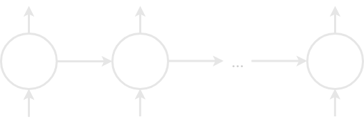
\(h_t=sigm(W^{hx}x_t+W^{hh}h_{t-1})\)

\(y_t=W^{yh}h_t\)

\(y_1\)

\(y_2\)

\(y_T\)

\(x_1\)

\(x_2\)

\(x_T\)

\(h_1\)

\(h_2\)

\(h_{T-1}\)

LSTM

• To estimate the conditional probability \(p(y_1, ..., y_{T'}|x_1, ..., x_T)\)
• \((x_1, ..., x_T)\) is an input sequence.
• \((y_1, ..., y_{T'})\) is its corresponding output sequence
• Length \(T'\) may differ from \(T\)
• \(v\) is the representation of \((x_1, ..., x_T)\)

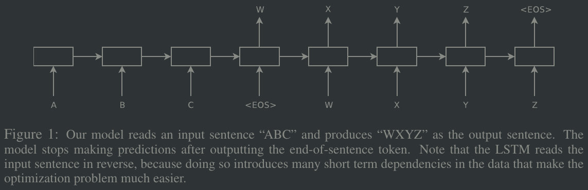
\(p(y_1, ..., y_{T'} | x_1, ..., x_T) = \displaystyle\prod_{t=1}^{T'}p(y_t|v, y_1, ..., y_{t-1})\)

Additional Preprocessing

• Require each sentence end with an EOS symbol.
  • For input {"A", "B", "C", "<EOS>"}, compute the probability of {"W", "X", "Y", "Z", "EOS"}.
• The performance is greatly boost when the input sentence is reversed.
  • For example \(a, b, c\) map to \(\alpha,\beta,\gamma\).
  • The LSTM is ask to map \(c,b,a\) to \(\alpha,\beta,\gamma\)

Additional to Model

• Two LSTM are different, so will make it able to train on multiple language pairs simultaneously.
• Deep is better then shallow, an LSTM with 4 layers is used.

Experiments

Dataset

• WMT'14 English to French dataset.
  • 12M sentences.
  • 348M French words.
  • 304M English words.
• Vocabulary of language models
  • 160,000 words for the source language.
  • 80,000 words for the target language.
  • OOV words was replaced with "UNK" token.

Decoding

• Maximizing the log probability of translation \(T\) given the source sentence \(S\).
• \(\mathcal{D}\) is the training set.

\(1/|\mathcal{D}|\displaystyle\sum_{(T,S)\in\mathcal{D}}\log p(T|S)\)

• Translations is produced by finding the most likely translation according to the equation.

\(\hat{T}=\arg\displaystyle\max_T p(T|S)\)

Decoding

• Search for the most likely translation using beam search decoder.
• Perform well even with a beam size of 1.

Rescoring

• Using the LSTM to rescore the 1000-best lists produced by the baseline system.
• Computed the log probability of every hypothesis with LSTM and took an even average with their score and the LSTM's score.

Reversing the Source Sentences

• LSTM learn much better with reversed source sentences.
• Perplexity dropped from 5.8 to 4.7.
• BLEU scores increased from 25.9 to 30.6.

\(c\)

\(b\)

\(a\)

\(\alpha\)

\(\beta\)

\(\gamma\)

\(c\)

\(b\)

\(a\)

\(\alpha\)

\(\beta\)

\(\gamma\)

Training Details

• LSTMs with 4 layers.
• 1000 cells at each layer.
• 1000 dimensional word embeddings.
• A native softmax over 80,000 words at each output.
• Initialized all of the LSTM's parameters with the uniform distribution between -0.08 and 0.08.
• Using SGD without momentum.

Training Details

• Fixed learning rate of 0.7.
• After 5 epochs, begin halving the learning rate every 0.5 epoch.
• Total of 7.5 epochs.
• Batches of 128 sequences for the gradient.
• Make sure that all sentences within a minibatch were roughly of the same length.

Parallelization

• Using 8-GPU machine.
• Each layer executed on a different GPU.
• Communicated its activations to the next GPU.
• The remaining 4 GPUs parallelize the softmax.
• Each GPU multiplying by a \(1000\times 20000\) matrix.
• 6,300 words per second with minibatch size of 128.
• Training took about 10 days.

Experimental Results

Score

• Use the cased BLEU score to evaluate.
• Compute by a perl script.
• Evaluate the state of the art system, got 37.0 which is greater than the 35.8 reported.

Tables

Method	Test BLEU Score (NTST14)
Bahdanau et al.	28.45
Baseline System	33.30
Single forward LSTM, beam size 12	26.17
Single reversed LSTM, beam size 12	30.59
Ensemble of 5 reversed LSTMs, beam size 1	33.00
Ensemble of 2 reversed LSTMs, beam size 12	33.27
Ensemble of 5 reversed LSTMs, beam size 2	34.50
Ensemble of 5 reversed LSTMs, beam size 12	34.81

Table 1: The performance of the LSTM on WMT'14 English to French test set (ntst14).

Tables

Method	Test BLEU Score (NTST14)
Baseline System	33.30
Cho et al.	34.54
State of the art	37.0
Rescoring the baseline 1000-best with a single forward LSTM	35.61
Rescoring the baseline 1000-best with a single reversed LSTM	35.85
Rescoring the baseline 1000-best with an ensemble of 5 reversed LSTMs	36.5
Oracle Rescoring of the Baseline 1000-best lists	~45

Table 2: Methods that use neural networks together with an SMT system.

Tables

Method	Test BLEU Score (NTST14)
Bahdanau et al.	28.45
Baseline System	33.30
Cho et al.	34.54
State of the art	37.00
Single forward LSTM, beam size 12	26.17
Single reversed LSTM, beam size 12	30.59
Ensemble of 5 reversed LSTMs, beam size 1	33.00
Ensemble of 2 reversed LSTMs, beam size 12	33.27
Ensemble of 5 reversed LSTMs, beam size 2	34.50
Ensemble of 5 reversed LSTMs, beam size 12	34.81
Rescoring the baseline 1000-best with a single forward LSTM	35.61
Rescoring the baseline 1000-best with a single reversed LSTM	35.85
Rescoring the baseline 1000-best with an ensemble of 5 reversed LSTMs	36.5
Oracle Rescoring of the Baseline 1000-best lists	~45

Model Analysis

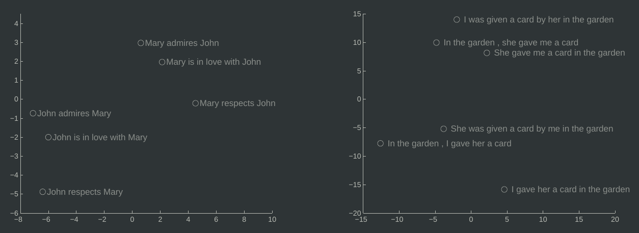
Figure 2: The 2-dimensional PCA projection of the LSTM hidden states that are obtained after processing the phrases in the figures.

Examples

...OAO

Figure

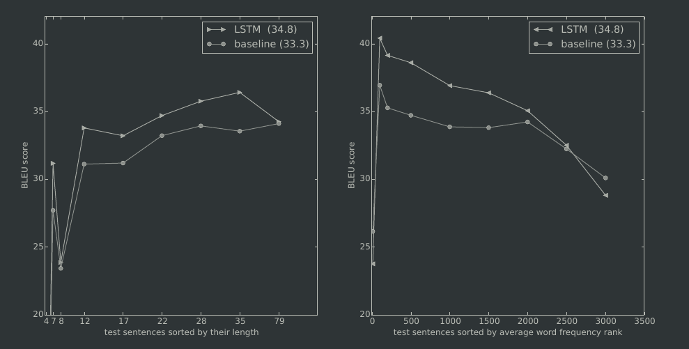
Figure 3: The left plot is showed with sorted by length of test sentences. The right plot is showed with sorted by average word frequency rank of test sentences.