

3DOR-2024
M
A
R
F
Towards Multi-View Consistency
in Neural Ray Fields
using Parametric Medial Surfaces
P
Parametric
Peder Bergebakken Sundt
Theoharis Theoharis
M
A
R
F
P
Parametric
3DOR-2024
Peder Bergebakken Sundt
Theoharis Theoharis
Towards Multi-View Consistency
in Neural Ray Fields
using Parametric Medial Surfaces
M
A
R
F
P
Medial
Atom
Ray
Field
Parametric
3DOR-2024
Peder Bergebakken Sundt
Theoharis Theoharis
Towards Multi-View Consistency
in Neural Ray Fields
using Parametric Medial Surfaces
A novel shape representation
Motivation
Fields
- Continuous
- Differentiable
- Different fields/signals are amenable to different novel applications
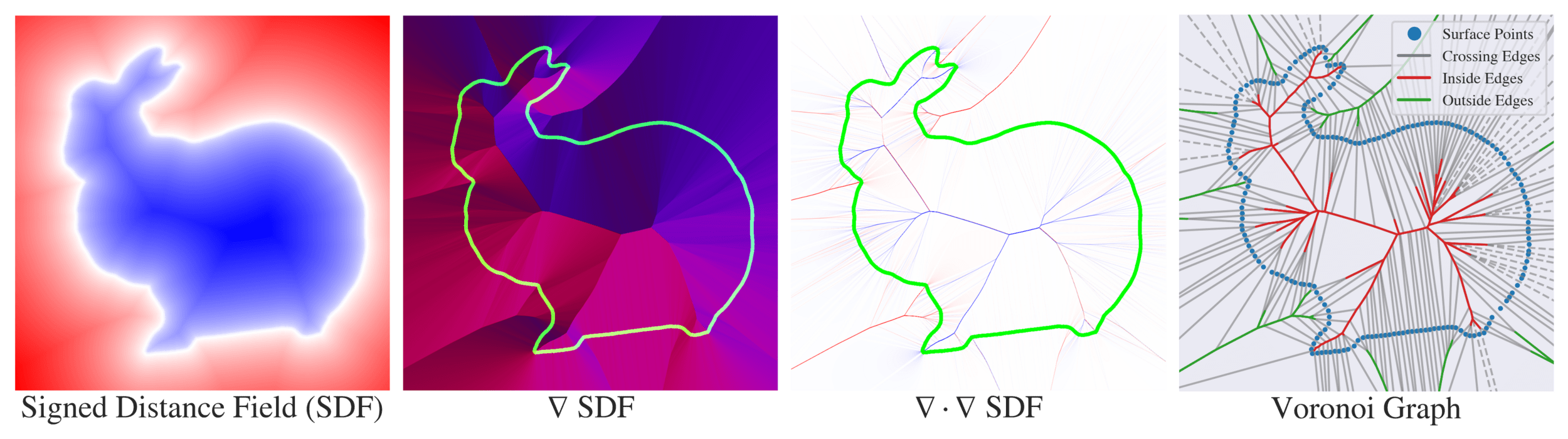
- Signed distance \(\to\) quick to traverse, watertight
- Generalized winding number \(\to\) self intersections, cloth
- Learned descriptor fields \(\to\) robotics
- Language embeddings \(\to\) semantic queries
\mathcal X\to\mathcal Y
\mathbb R ^3\to[0,1]
Why make novel Neural Fields?
- Effective in Inverse Rendering and other problems in Visual Computing
like analysis-by-synthesis-
High compression ability
-
Able to learn mappings
previously considered ill-posed
(lottery ticket hypothesis)
-
-
New mappings enable new applications
Why ray fields?
Neural fields are great at solving inverse rendering, but are slow to render
Directly predict
ray integral
Why ray fields?
Neural fields are great at solving inverse rendering, but are slow to render
Offline Tabulation
Precompute samples,
discretization artifacts (aliasing)
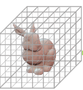
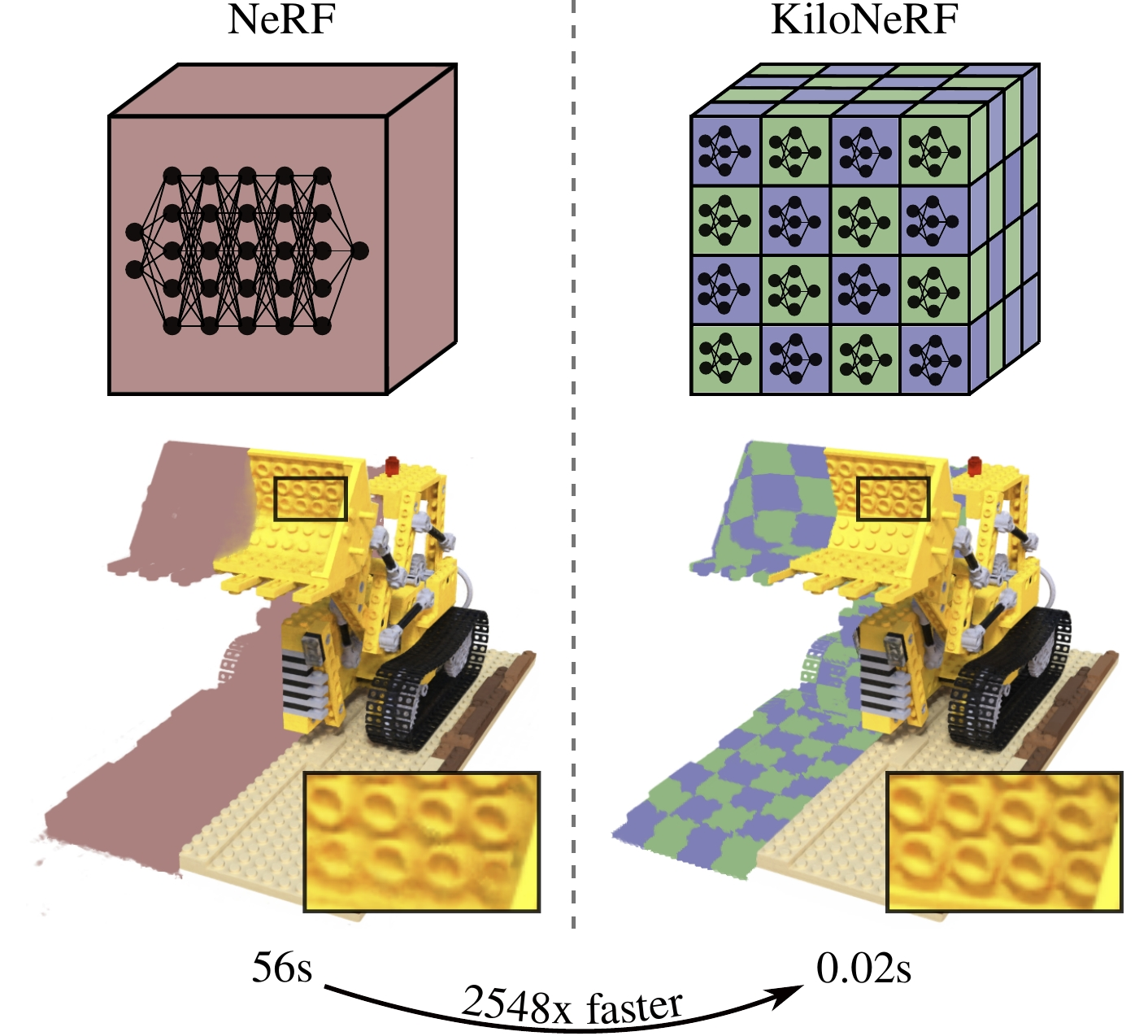
Hybrid methods
(Many small networks)
Cheaper samples, trade compute for memory, loss of global shape prior
Gaussian splatting
100x, View-dependent, no notion of surface or prior, hard to extract geometry
Learn heuristic field
(SDF)
10x reduction in samples, no transparent objects
Directly predict
ray integral
Neural fields are great at solving inverse rendering, but are slow to render
Why ray fields?

100x, View-
dependent, can represent both color and geometry, less studied
Offline Tabulation
Precompute samples,
discretization artifacts (aliasing)
Hybrid methods
(Many small networks)
Cheaper samples, trade compute for memory, loss of global shape prior
Gaussian splatting
100x, View-dependent, no notion of surface or prior, hard to extract geometry
Learn heuristic field
(SDF)
10x reduction in samples, no transparent objects
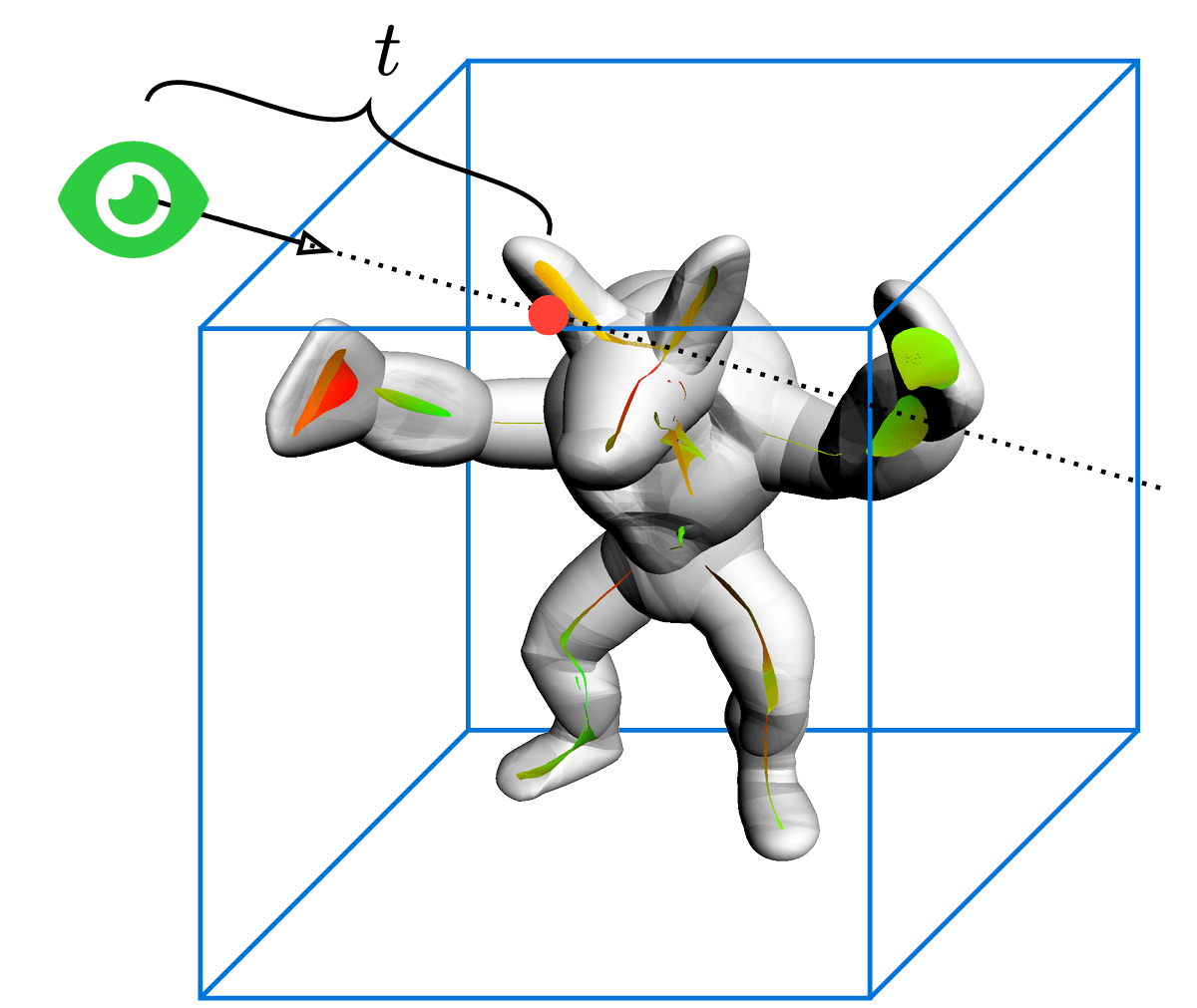
Cartesian Field functions (\(\mathbb R^3\to\mathcal X\))
require multiple sample along ray
While Ray Field functions (\(\mathcal R\to\mathcal X\))
map directly to the result
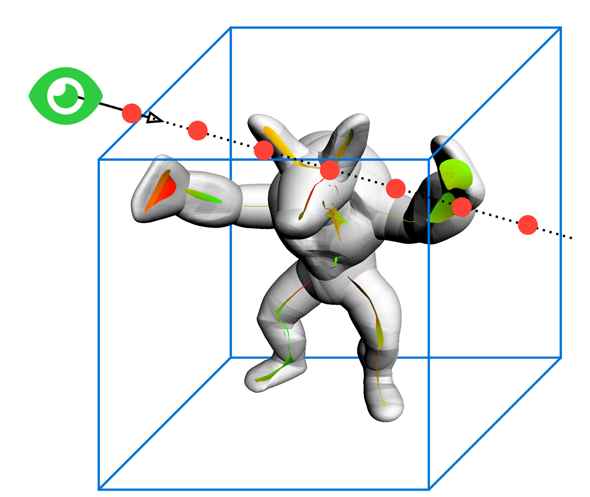
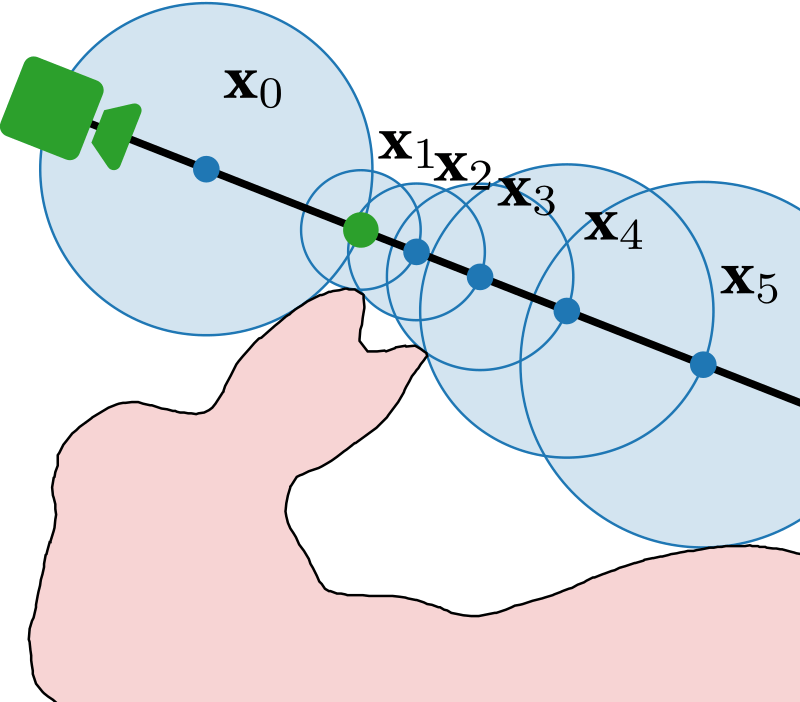
We build on the Medial Atom Ray Field (MARF)
Why build on MARF?
- Deals with ray field discontinuities
(Lipschitz bound) - Inherent multi-view consistency in reconstruction domain
- Emit cheap surface normals
Why build on MARF?
\bigg\}
- Deals with ray field discontinuities
(Lipschitz bound) - Inherent multi-view consistency in reconstruction domain
- Emit cheap surface normals
Background


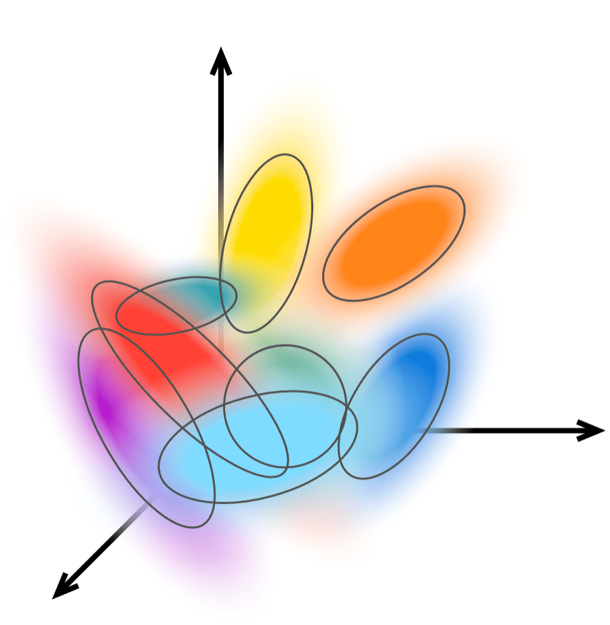
"Medial axis"
Set of maximally inscribed spheres
"Medial axis"
The set of maximally inscribed spheres, or "atoms"
Ridges of the distance transform
"Medial axis"
Ridges of the distance transform
The set of maximally inscribed spheres, or atoms
Set of points with two nearest neighbors
"Medial axis"
Set of points with two nearest neighbors
Ridges of the distance transform
Set of points with two nearest neighbors
"Medial axis"
\ell
\ell
\ell
\{
\mathbf x_i, r_i
\}_{i=1}^k
\rightarrow
\ell
\mathbf x_1, r_1
MARF
\mathbf x_2, r_2
\mathbf x_4, r_4
\mathbf x_3, r_3
\ell
\{
\mathbf x_i, r_i
\}_{i=1}^k
\rightarrow
\ell
\mathbf x_1, r_1
MARF
\mathbf x_2, r_2
\mathbf x_4, r_4
\mathbf x_3, r_3
\mathbf x_2, r_2
\mathbf x_2, r_2
\ell
\mathbf x_i, r_i
\mapsto
?
\mathbf x_2, r_2
\ell
\mathbf x_i, r_i
\mapsto
\mathbb R^3\times \mathbb R^+
\rightarrow
S^2\times \mathbb R ^2
(4 DoF)
\rightarrow
\mathbb R^2
(4 DoF)
?
View direction + xy in view plane
Atom/sphere
MARF
P
\mathbf x_2, r_2
\ell
\mathbf x_i, r_i
\mapsto
\mathbb R^3\times \mathbb R^+
\rightarrow
S^2\times \mathbb R ^2
(4 DoF)
\rightarrow
\mathbb R^2
(4 DoF)
2 DoF!
Parametric surface
MARF
P
f_i:\begin{cases}
\ell &\to \mathbb R ^3\times\mathbb R^+ \\
(\mathbf x, \hat{\mathbf q}) & \mapsto
\end{cases}
(u_i, v_i)
(x_i, y_i, z_i, r_i)
g_i:\begin{cases}
\mathbb R ^2 &\to \mathbb R ^3\times\mathbb R^+ \\
(u_i, v_i) & \mapsto
\end{cases}
Zero Thickness by construction
More accurate medial surface
\(\Rightarrow\) More stable atoms
f_i:\begin{cases}
\ell &\to \mathbb R ^3\times\mathbb R^+ \\
(\mathbf x, \hat{\mathbf q}) & \mapsto
\end{cases}
(u_i, v_i)
(x_i, y_i, z_i, r_i)
Architecture

MARF
P
Prior work
Ours
MARF
P
Prior work
Ours
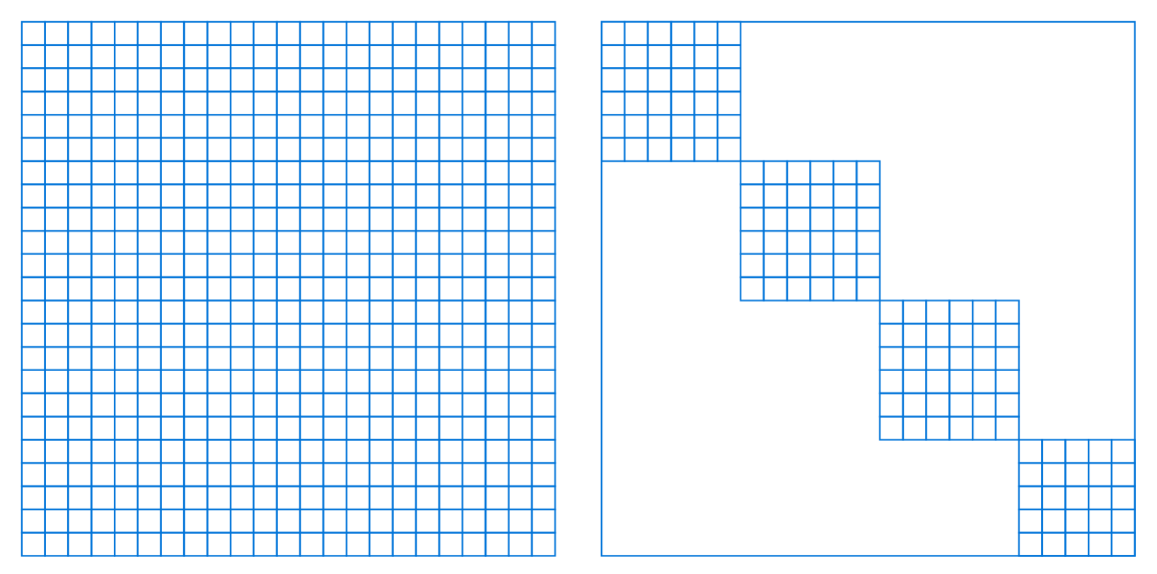
Multiple MLP Heads
Block-diagonal matrices
Batched matrix multiplication
MARF
P
Prior work
Ours
Multiple MLP Heads
Block-diagonal matrices
Batched matrix multiplication
MARF
P
Prior work
Ours
Multiple MLP Heads
Block-diagonal matrices
Batched matrix multiplication
Fewer weights
Block diagonal
Fewer weights
Fully connected
Fewer weights
Block diagonal
Fully connected
Batched Matrix
Fewer weights
Block diagonal
Fully connected
Batched Matrix
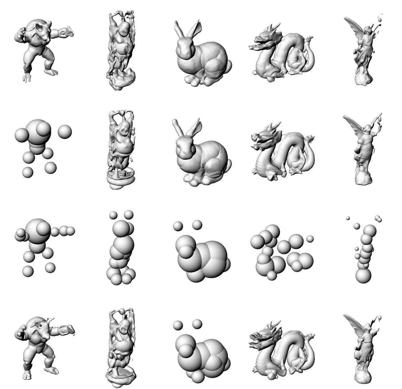
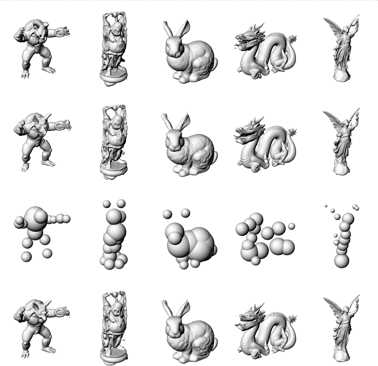
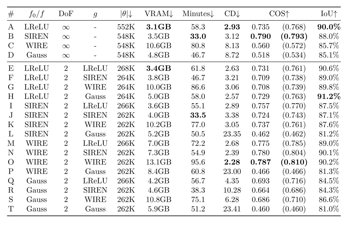
We evaluate 4 different activations/nonlinearities
Evaluation
[1] Ba JL, Kiros JR, Hinton GE. Layer Normalization 2016.
[3] Ramasinghe S, Lucey S. Beyond Periodicity: Towards a Unifying Framework for Activations in Coordinate-MLPs. In: Avidan S, Brostow G, Cissé M, Farinella GM, Hassner T, editors. Computer Vision – ECCV 2022, Cham: Springer Nature Switzerland; 2022, p. 142–58.
[2] Sitzmann V, Martel JNP, Bergman AW, Lindell DB, Wetzstein G. Implicit Neural Representations with Periodic Activation Functions. Proc. NeurIPS, 2020
[4] Saragadam V, LeJeune D, Tan J, Balakrishnan G, Veeraraghavan A, Baraniuk RG. WIRE: Wavelet Implicit Neural Representations, 2023, p. 18507–16

ReLU [1]

SIREN [2]

Gauss [3]

WIRE [4]
We evaluate 4 different activations/nonlinearities
Evaluation
First we try each on the prior architecture
ReLU [1]
SIREN [2]
Gauss [3]
WIRE [4]
Ground
Truth
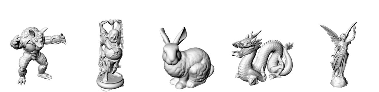
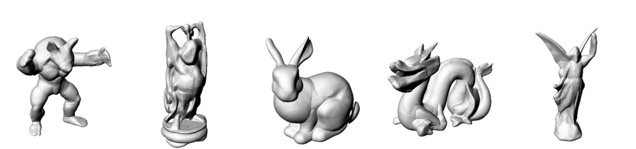
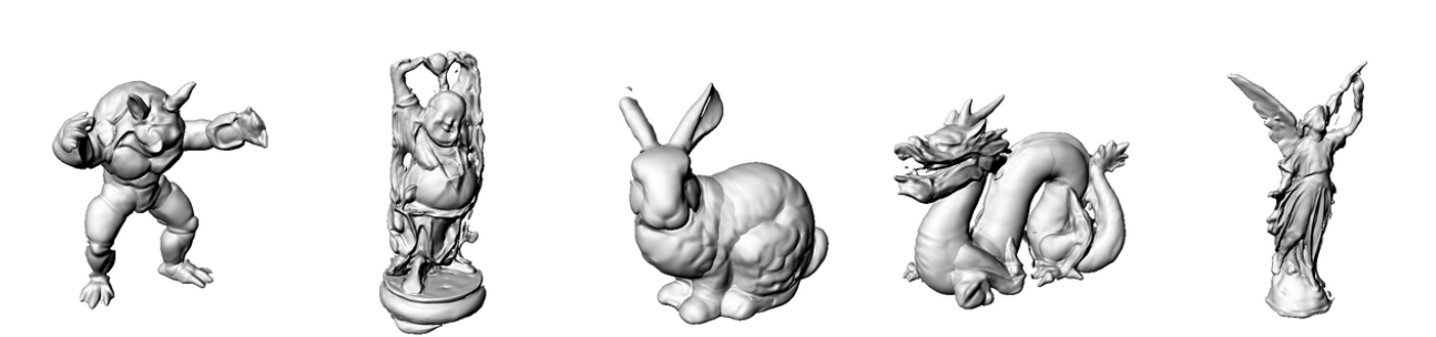
ReLU [1]
SIREN [2]
Gauss [3]
WIRE [4]
Ground
Truth
\times
\times
\times
\times
ReLU [1]
ReLU [1]
ReLU [1]
ReLU [1]
Ray decoder
Surface decoder
ReLU [1]
SIREN [2]
Gauss [3]
WIRE [4]
Ground
Truth
\times
\times
\times
\times
ReLU [1]
ReLU [1]
ReLU [1]
ReLU [1]
Ray decoder
WIRE [4]
Surface decoder
ReLU [1]
ReLU [1]
SIREN [2]
Gauss [3]
WIRE [4]
Ground
Truth
ReLU [1]
\times
ReLU [1]
ReLU [1]
ReLU [1]
\times
\times
\times
SIREN [2]
SIREN [2]
SIREN [2]
SIREN [2]
Ray decoder
WIRE [4]
Surface decoder
ReLU [1]
ReLU [1]
SIREN [2]
Gauss [3]
WIRE [4]
Ground
Truth
ReLU [1]
\times
ReLU [1]
ReLU [1]
ReLU [1]
\times
\times
\times
SIREN [2]
SIREN [2]
SIREN [2]
SIREN [2]
ReLU [1]
ReLU [1]
SIREN [2]
Gauss [3]
WIRE [4]
Ground
Truth
ReLU [1]
\times
ReLU [1]
ReLU [1]
ReLU [1]
\times
\times
\times
SIREN [2]
SIREN [2]
SIREN [2]
SIREN [2]
Gauss [3]
Gauss [3]
Gauss [3]
Gauss [3]
ReLU [1]
SIREN [2]
Gauss [3]
WIRE [4]
Ground
Truth
\times
\times
\times
\times
SIREN [2]
SIREN [2]
SIREN [2]
SIREN [2]
Gauss [3]
Gauss [3]
Gauss [3]
Gauss [3]
WIRE [4]
WIRE [4]
WIRE [4]
WIRE [4]
ReLU [1]
SIREN [2]
Gauss [3]
WIRE [4]
Ground
Truth
\times
\times
\times
\times
Gauss [3]
Gauss [3]
Gauss [3]
Gauss [3]
WIRE [4]
WIRE [4]
WIRE [4]
WIRE [4]
ReLU [1]
SIREN [2]
Gauss [3]
WIRE [4]
Ground
Truth
\times
\times
\times
\times
Gauss [3]
WIRE [4]
WIRE [4]
WIRE [4]
WIRE [4]
\bigg\}
MARF
arch is
unstable
\bigg\}
\bigg\}
MARF
arch is
unstable
\bigg\}
\bigg\}
MARF
arch is
unstable
\bigg\}
>>> # (BATCH, N_BLOCKS, INTER-BLOCK WIDTH)
>>> input = torch.empty(128, 8, 8)
>>> weight = torch.empty(8, 8, 8)
>>> output = torch.einsum("...ij,ijk->...ik", input, weight)
>>> output.shape
torch.Size([128, 8, 8])
>>> output.stride()
(8, 1024, 1)
>>> torch.empty(128, 8, 8).stride()
(64, 8, 1)
>>> # (BATCH, N_BLOCKS, INTER-BLOCK WIDTH)
>>> input = torch.empty(128, 8, 8)
>>> weight = torch.empty(8, 8, 8)
>>> output = torch.einsum("...ij,ijk->...ik", input, weight)
>>> output.shape
torch.Size([128, 8, 8])
>>> output.stride()
(8, 1024, 1)
>>> torch.empty(128, 8, 8).stride()
(64, 8, 1)
>>> # (BATCH, N_BLOCKS, INTER-BLOCK WIDTH)
>>> input = torch.empty(128, 8, 8)
>>> weight = torch.empty(8, 8, 8)
>>> output = torch.einsum("...ij,ijk->...ik", input, weight)
>>> output.shape
torch.Size([128, 8, 8])
>>> output.stride()
(8, 1024, 1)
>>> torch.empty(128, 8, 8).stride()
(64, 8, 1)
>>> torch.tensor( 1 + 2j ).to(torch.float16)
UserWarning: Casting complex values to real discards the imaginary part

tensor(1., dtype=torch.float16)
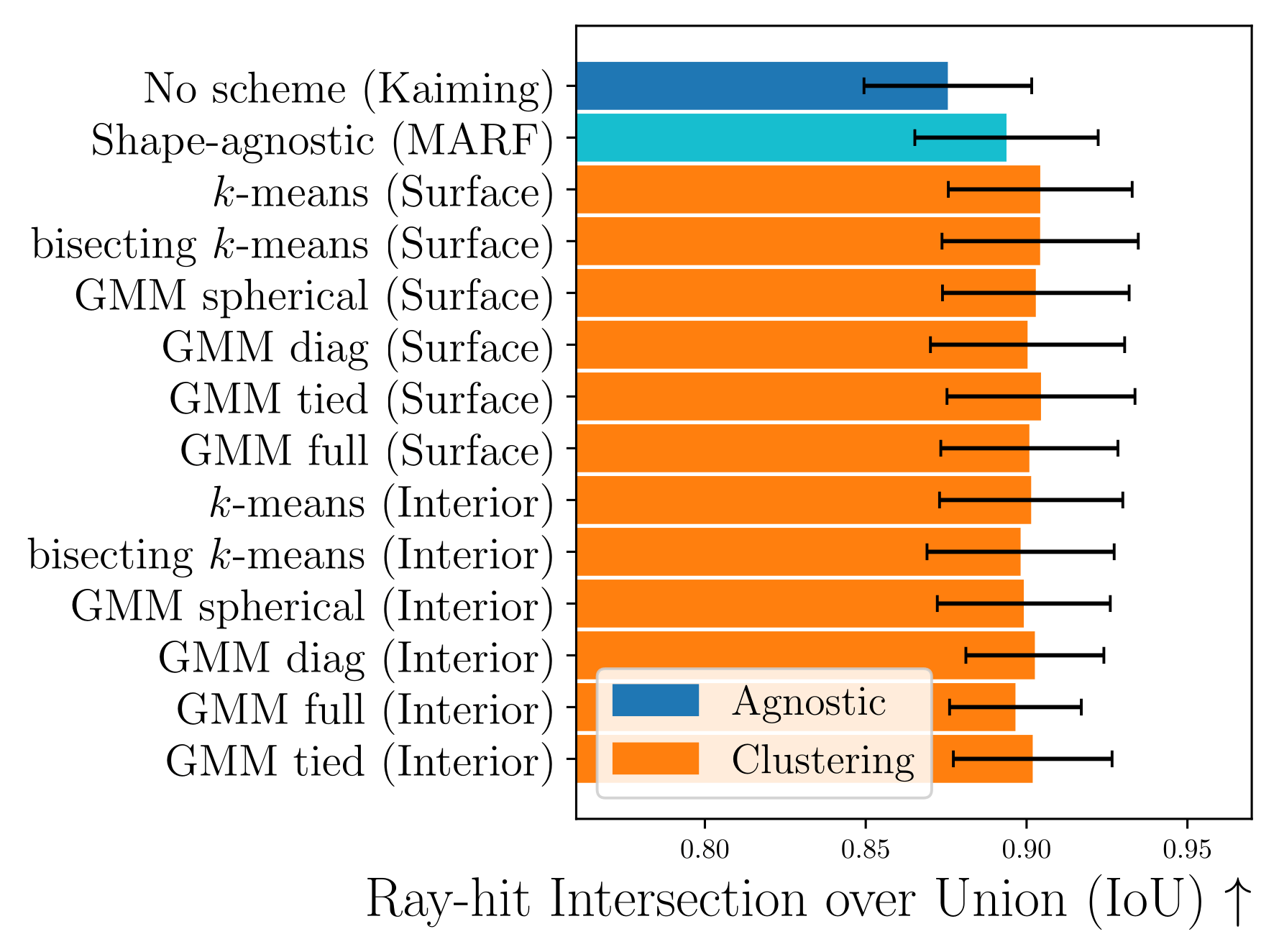
Initialization
Surface points
Surface clouds are simple to compute from depth scans or SfM landmarks
Surface points
Agnostic (MARF)
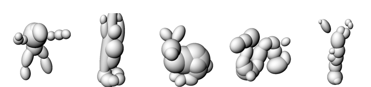
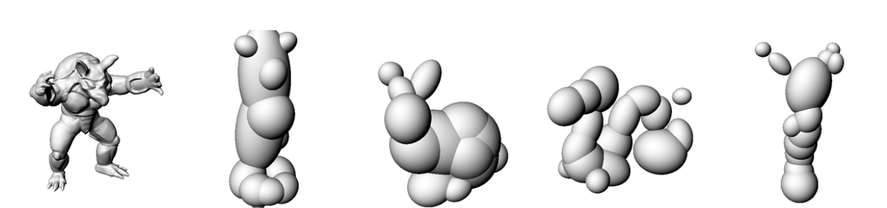
K-Means Clustering (Ours)
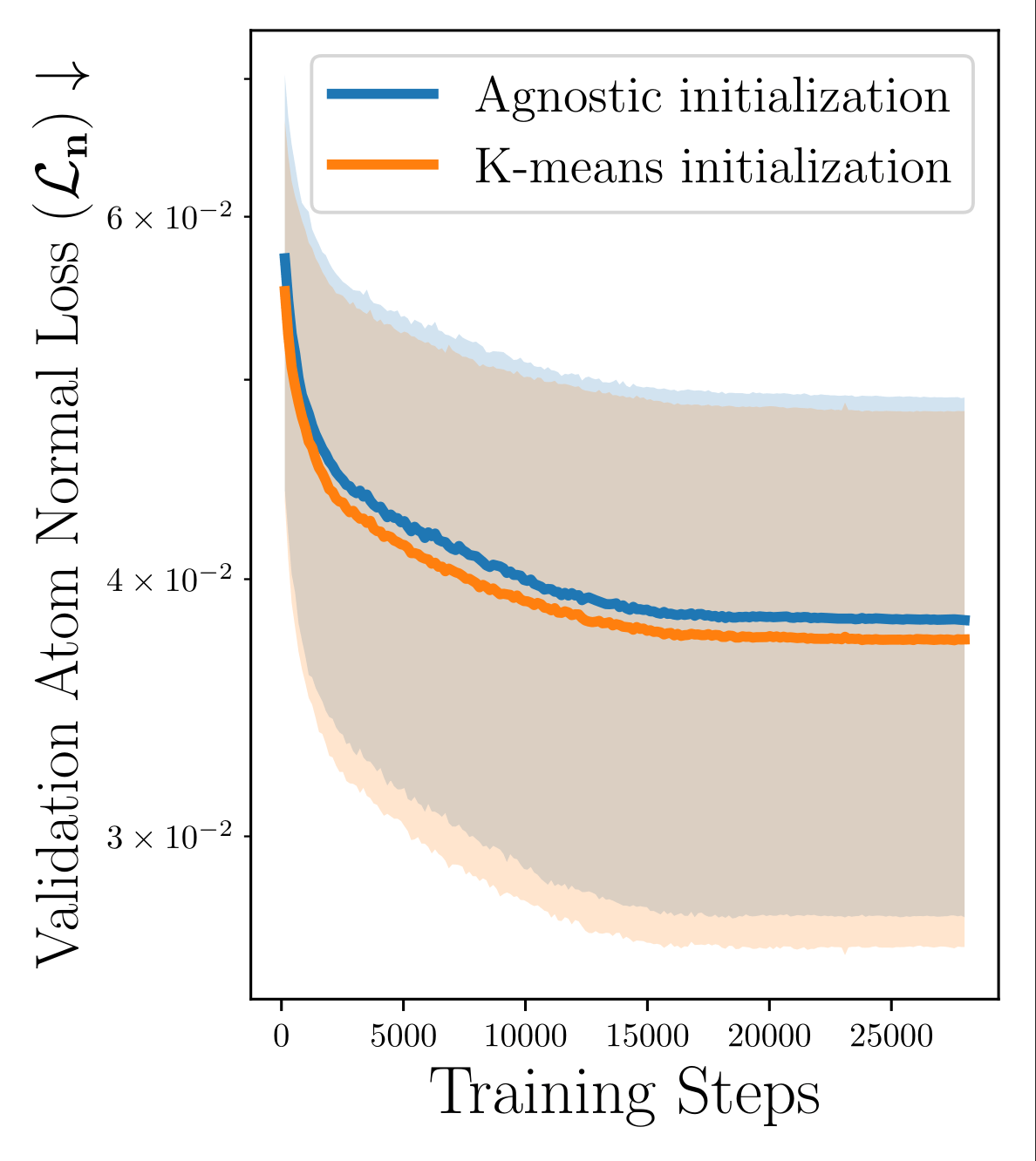
Average over 80 runs, for each shape activation function
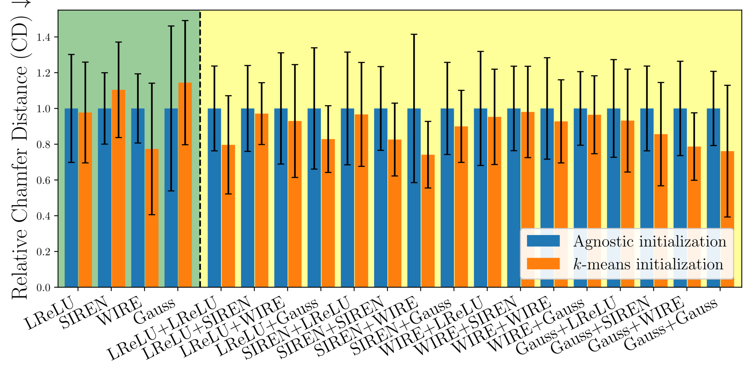
MARFs
PMARFs
Non-ReLU
too unstable
to get a good read
Strict improvement
Exploring various unsupervised clustering algorithms
Surface points
Interior Volume points
(Requires full view, and is too expensive to compute in a real-time scenario)
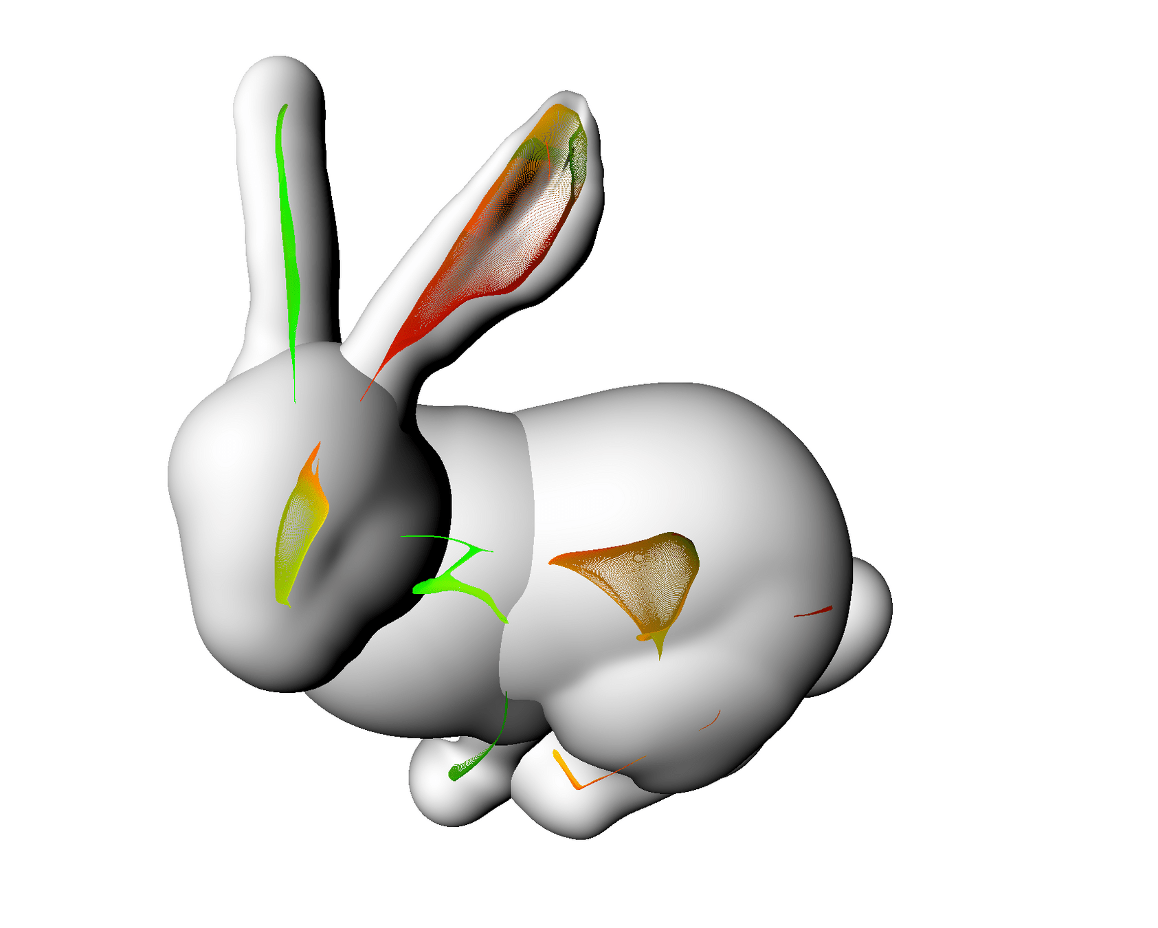
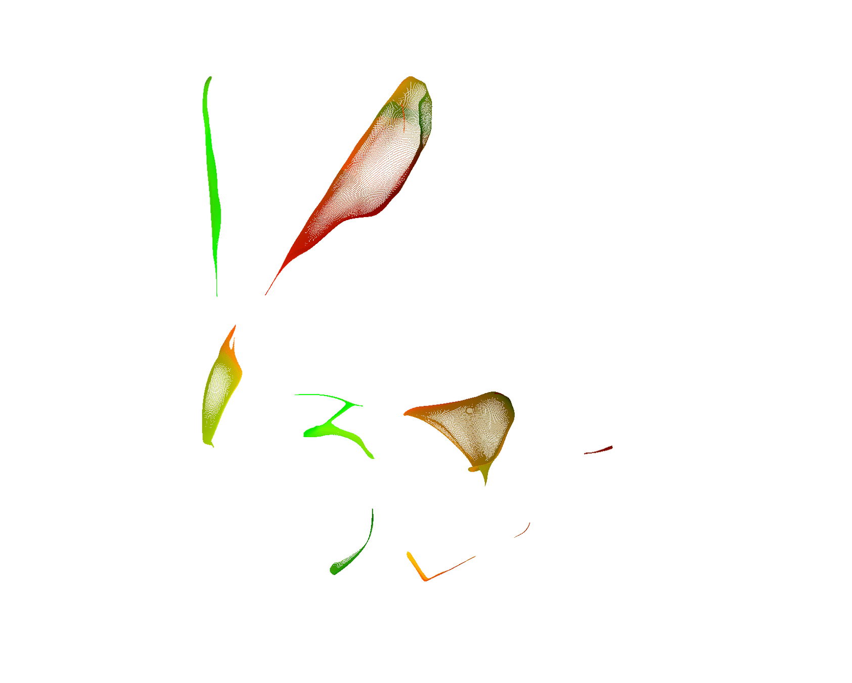
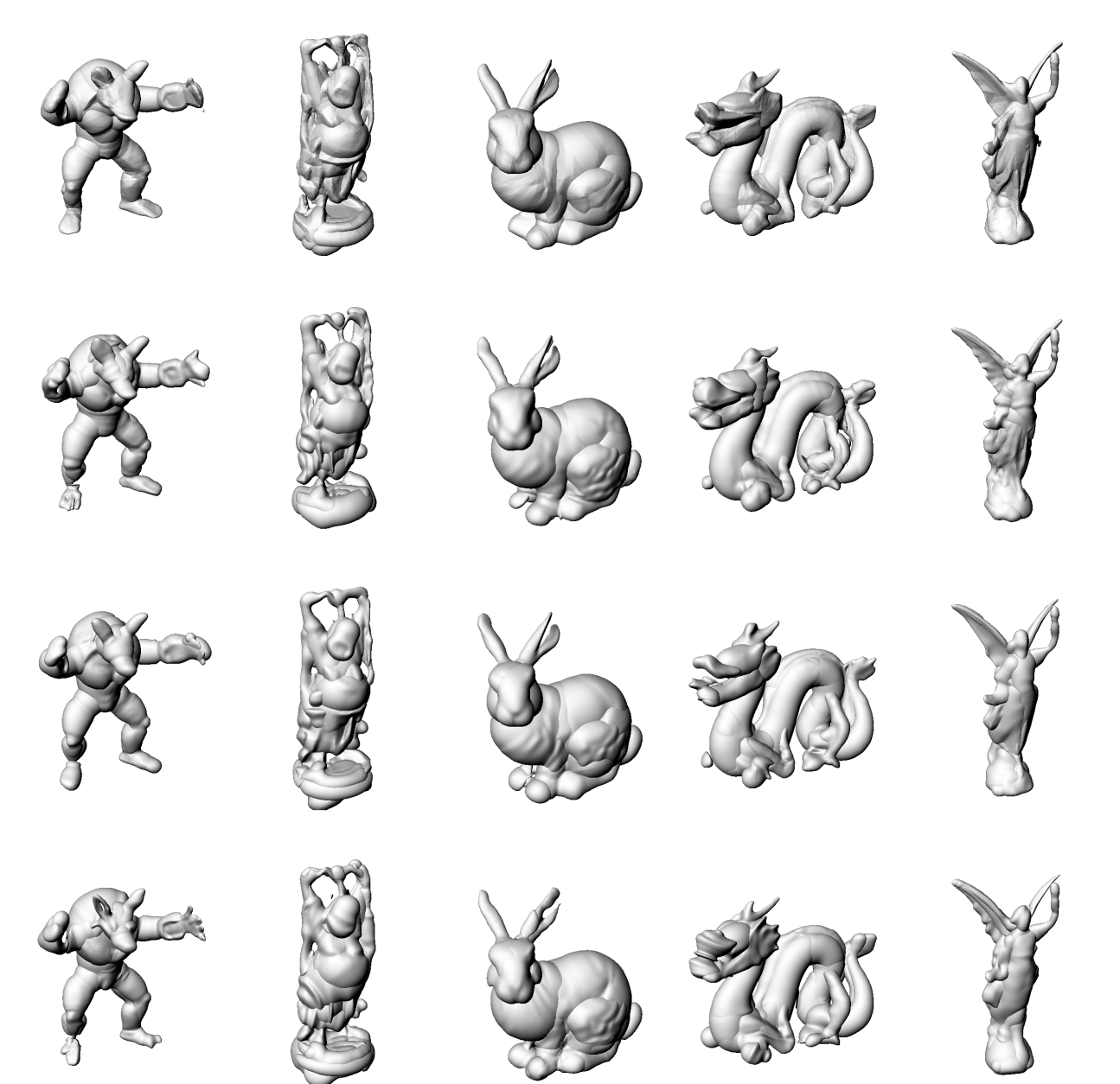
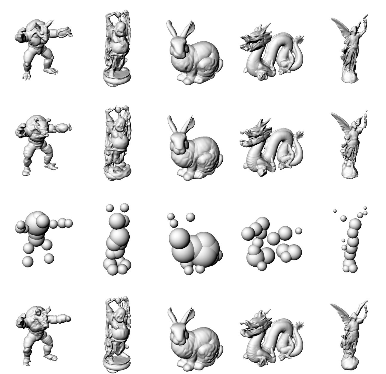
Sparse-view Scenarios
35 training views, 15 validation views
~4000 test views
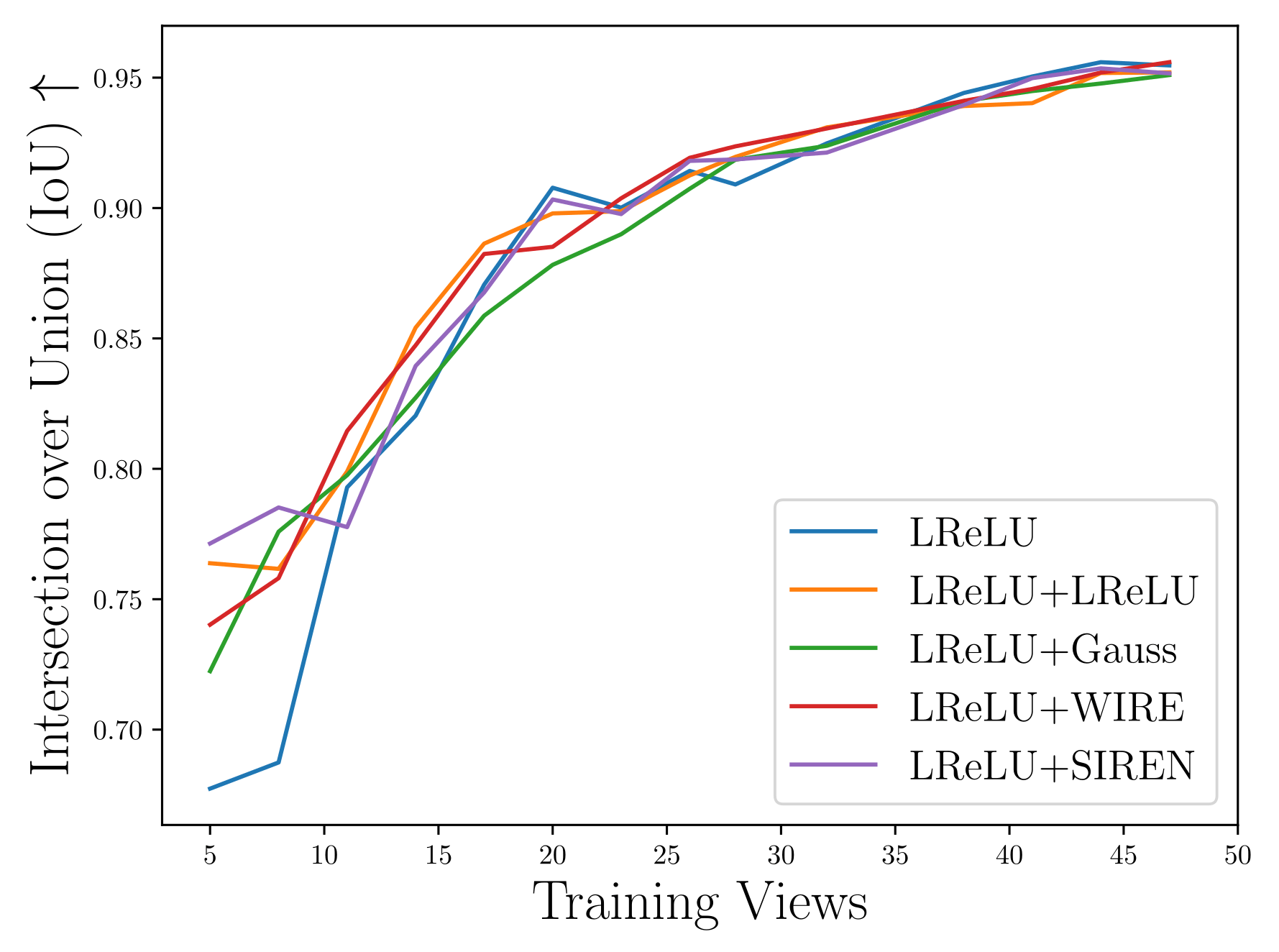
Sparse-view Scenarios
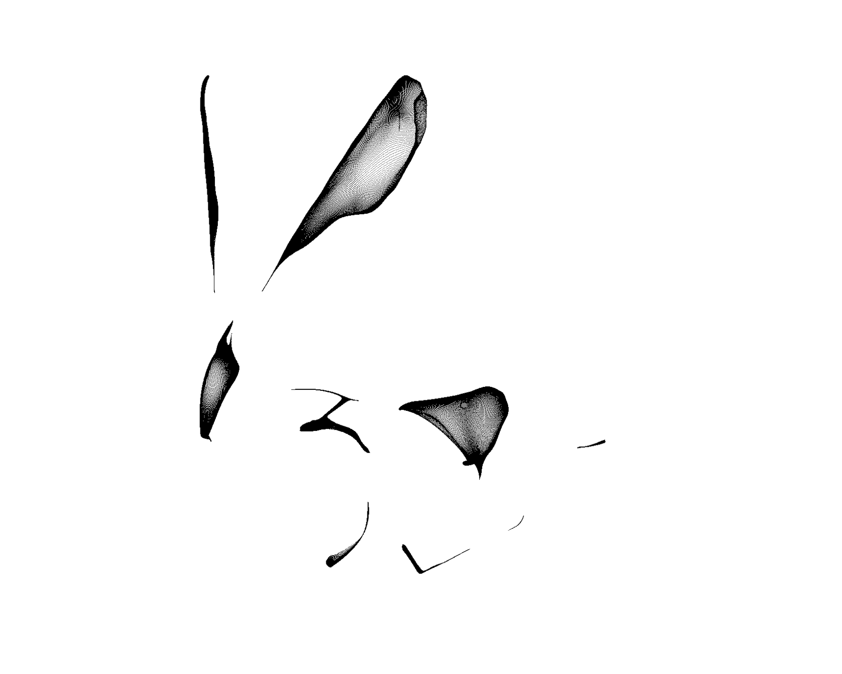
PMARFs
MARF
Sparse-view Scenarios
Conclusion
We present PMARF a Neural Ray Field with
- Improved multi-view consistency
- Improved reconstruction fidelity
- A lower parameter count, and that
- Performs well with more advanced nonlinearities
Thank you
Questions?
PMARF
By pbsds


