Modeling Real-Time Stocks Using Monte Carlo Simulations
Presented by:
Keyur Chaudhari
Prabhas Reddy Onteru
Shruti Goswami
Problem Statement
- The stock market is a dynamic system influenced by numerous factors.
- Accurate predictions can reduce investment risk by helping investors make informed decisions.
- Objective: Model and forecast stock prices using Monte Carlo simulations.
- Goal: Provide insights to aid in risk assessment and strategic investment.
Related Work
-
ARIMA:
-
Best for short-term; limited in capturing long-term trends.
-
Assumes linearity, struggles with stock market volatility.
-
-
Markov Chains:
-
Assumes future depends only on the current state, ignoring past events.
-
Can't model long-term patterns and sudden drifts in stocks effectively.
-
Traditional Methods:
Deep Learning Methods (e.g., LSTM, Neural Networks):
-
Interpretability Issues : Often a “black box,” limiting transparency for financial strategy and risk assessment.
-
Hyperparameter Sensitivity : Demands time-consuming tuning for optimal performance.
-
Computationally Expensive : Requires high-performance hardware and large datasets, which increases cost.
Methodology: ARIMA Model
-
If the series is non-stationary, differencing (using Integrated terms) can be applied to make the series stationary.
-
Autoregressive (AR) terms: Models the relationship between an observation and its previous values.
-
This can be expressed as:
-
\(Y_t = c + \phi_1 Y_{t-1} + \phi_2 Y_{t-2} + \cdots + \phi_p Y_{t-p} + \epsilon_t\)
-
-
where \(Y_{t}\) is the current value, \(\phi_1, \ldots, \phi_p\)
are the autoregressive coefficients, and \(ϵ_{t}\) is white noise -
Similarly Moving Average terms models relationship between an observation and error terms.
-
We have used statsmodels.tsa.arima.model to automatically find ARIMA parameters that best fit the data.
Figure 1 : Original Data Plot
reference : https://neptune.ai/blog/arima-sarima-real-world-time-series-forecasting-guide
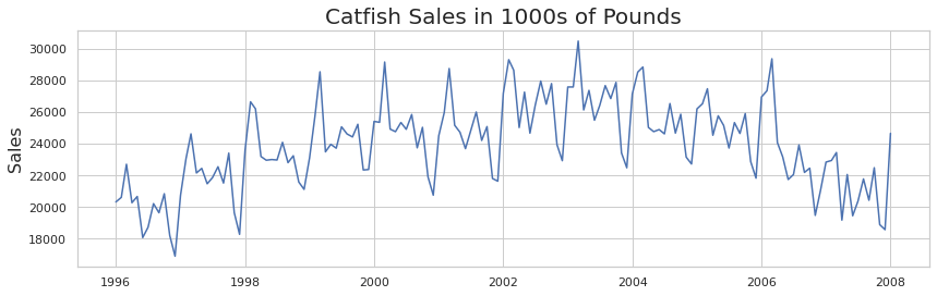
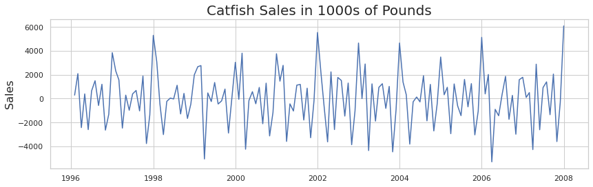
Figure 2 : Plot With d=1(differencing factor)
Methodology: Markov Chain Modeling
Methodology: LSTM Network
-
Training:
- LSTM can capture both short-term and long-term dependencies.
- Unlike RNNs which use only hidden states to pass information from previous states, LSTM utilizes Forget, Input, and Output gates for optimal data flow over time
-
Prediction:
- Given some history of prices, the prices will be passed through learned parameters to get output predictions.
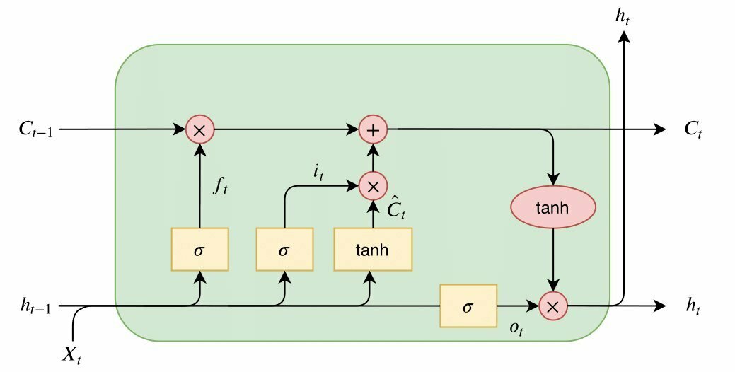
reference : https://thorirmar.com/post/insight_into_lstm/
Figure 3 : LSTM Cell
Methodology: Monte Carlo Simulation
-
Monte Carlo Simulation generates multiple future price paths where each one is random walk and uses these simulations to get predictions for the random variable associated.
-
Geometric Brownian Motion (GBM): Geometric Brownian Motion (GBM) is a stochastic process widely used for modeling stock prices. It assumes that the logarithm of the stock price follows a Brownian motion with drift.
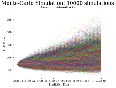
Figure 4 : 100K Simulations on APPL Dataset
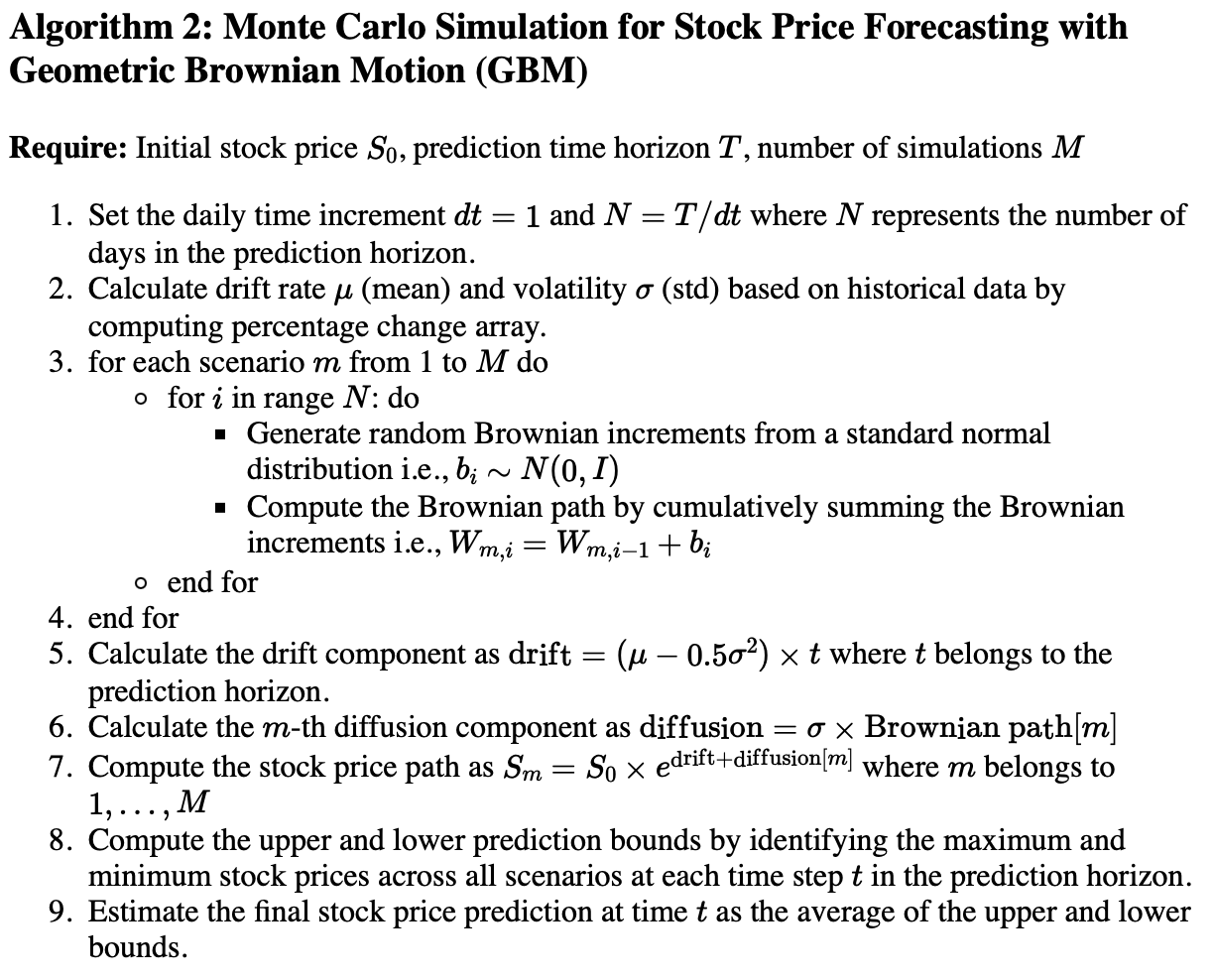
Algorithm for GBM
Results
- We have considered AAPL dataset obtained from Yahoo Finance (yfinance) which represents the APPLE stocks
| Dataset | Training Period | Testing period |
|---|---|---|
| Dataset-A | 2015-2020 | 2020-2021 |
| Dataset-B | 2015 to Oct 2020 | Nov 2020 to March 2021 |
Table 2 : Simulation Results For Different Sample Sizes On DATASET-A
| Simulation Size | MSE | MAE | RMSE |
|---|---|---|---|
| 100 | 249.83 | 16.33 | 18.70 |
| 100k | 150.66 | 9.29 | 12.27 |
| 50k | 340.26 | 18.12 | 20.98 |
Table 1 : Different Datasets considered
- The simulation results indicate that there need not be positive correlation between number of simulations and performance. So we have looped through all number of simulations with step size of 100 and reported the best obtained.
| Model | MSE | MAE | RMSE | Total Time |
|---|---|---|---|---|
| ARIMA | 1310.78 | 29.08 | 36.20 | 10 sec |
| Markov | 187.09 | 12.05 | 13.93 | 40 Sec |
| LSTM | 61.40 | 4.99 | 5.89 | 1 Hour 10 Min |
| GBM | 150.66 | 9.29 | 12.27 | 1 Min |
| Model | MSE | MAE | RMSE |
|---|---|---|---|
| ARIMA | 156.43 | 9.94 | 12.51 |
| Markov | 283.57 | 14.68 | 16.84 |
| LSTM | 25.72 | 4.17 | 5.07 |
| GBM | 73.64 | 6.52 | 8.58 |
Table 3 : Dataset-A results
Table 4 : Dataset-B results
Results
Comparison
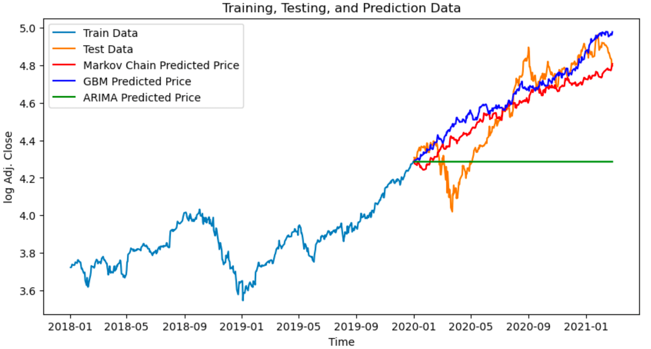
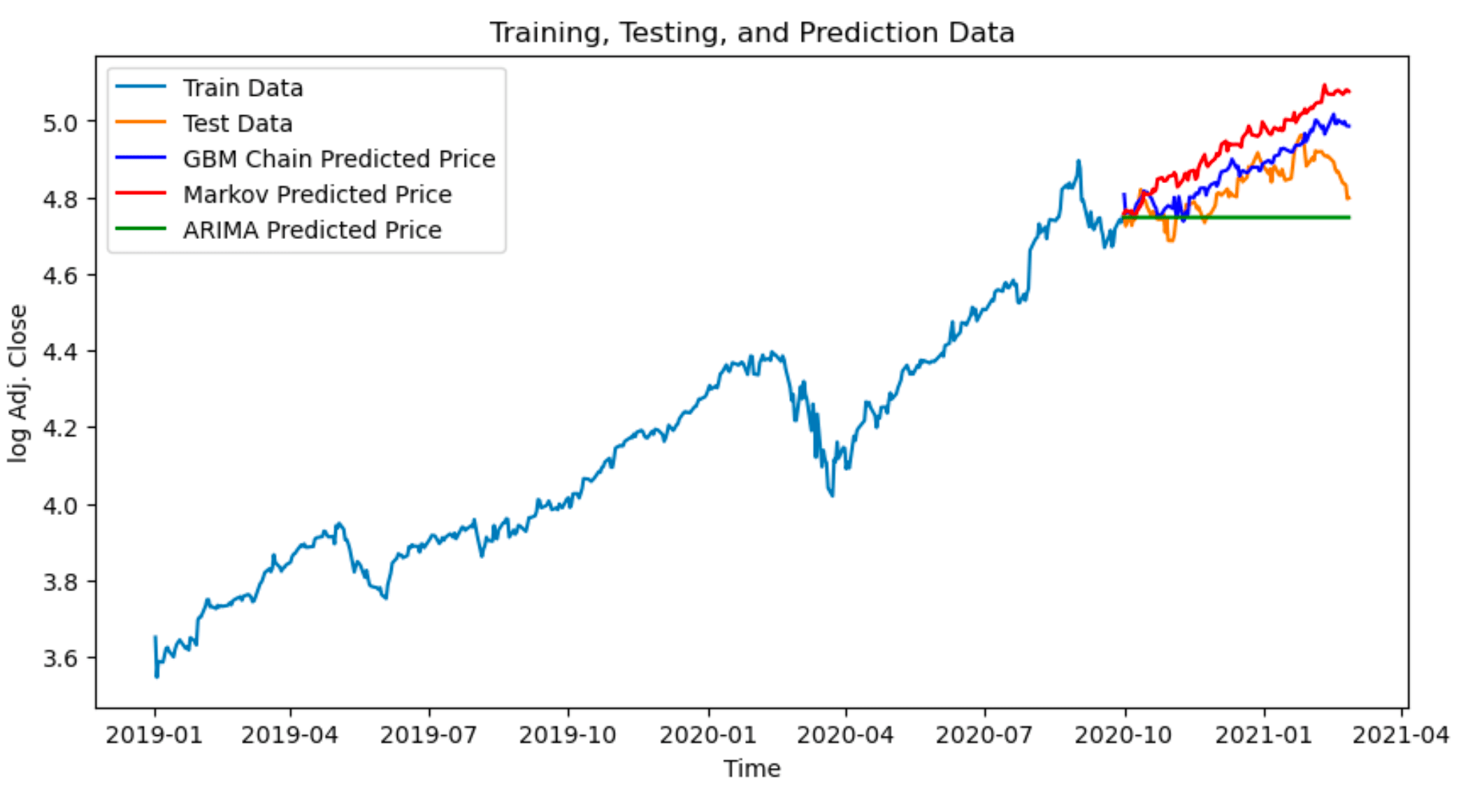
Figure 5 : Comparison of predictions of multiple methods over Dataset-A
Figure 6 : Comparison of predictions of multiple methods over Dataset-B
Conclusions
-
ARIMA tends to perform worst as it cannot handle non linearities present in stock data.
-
Monte Carlo simulations have performed well compared to other methods like ARIMA and Markov models.
-
However, LSTM models show better results when more parameters are used, making them more effective at capturing complex stock price patterns in certain cases.
-
But we can see Monte Carlo Simulations as a trade off between the performance and Computation.
Modeling_ppt
By PRABHAS ONTERU


