Active Reinforcement Learning Strategies for Offline Policy Improvement with

Cost-Aware Optimization

Presented by:

Prabhas Reddy Onteru

Guided by Prof.Ambedkar Dukkipati

June 16, 2025

Agenda

Background​

​

• This offline dataset will be of the form
                \[D = \left\{ (s_i, a_i, s'_i, r_i, d_i) \right\}_{1 \leq i \leq N}\]
• where \( s'_i \) is the next state resulting from taking action \( a_i \) in state \( s_i \), \( r_i \) is the corresponding reward, and \( d_i \) indicates whether the episode terminated.
• The goal of Offline Reinforcement Learning is to train an effective policy from this pre-collected dataset without further interactions.

Background​

​​

• In practice, learned policies may be sub-optimal, and agents are often allowed limited, cost-constrained interactions with the environment to collect additional trajectories.

• For instance, in autonomous vehicles, the budget may correspond to fuel consumption, while for robotic agents, it may involve constraints such as time and effort.

Problem Statement

• In this respect, the following learning problems emerge.
• (Q1) How does the agent learn to choose the additional trajectories to enhance the existing offline dataset and improve the current policy?
• (Q2) What sequence should the agent learn to collect these additional trajectories to make the most effective use of the agent’s budget?

Problem Statement

• Consider the following MDP \(\mathcal{M}_{\text{Act}} = (\mathcal{S}, \mathcal{A}, \mathcal{T}, r, \hat{\rho}, \gamma)\), with a different initial state distribution \(\hat{\rho}\) for the active trajectory collection phase.

• At the start of each episode, a set of candidate initial states \(\mathcal{C} = \{ s_i \sim \hat{\rho} : 1 \leq i \leq N \}\) is sampled from \(\hat{\rho}\). The agent can choose to begin exploring the environment from any subset of these candidates, and can also stop exploring at any time, if necessary, to preserve its budget.

Problem Setting

• The objective of the agent is to collect new samples , so as to maximize the performance in the original MDP \( \mathcal{M} \) of the policy trained on the resulting augmented dataset.

Objective

• (Q1) How does the agent learn to choose the additional trajectories to enhance the existing offline dataset and improve the current policy?

• The idea is to train an ensemble of \( k \) independent encoders: \( \{ E^i_s \}_{i=1}^k \), which map states \( s \) to a latent space, and \( \{ E^i_{s,a} \}_{i=1}^k \), which map state-action pairs \( (s, a) \) to a latent space.
• Training is performed using contrastive learning, where the anchor is a state \( s \), the positive sample is the next state \( s' \), and the negative sample is a random state \( s'' \). The corresponding embeddings are defined as \( v = E_s(s) \), \( v^+ = E_s(s') \), and \( v^- = E_s(s'') \).
• Additionally, a transition-consistent embedding \( \hat{v}^+ = E_{s,a}(s, a) \) is computed, which is encouraged to align with \( v^+ \)

Uncertanity models

• The training objective combines contrastive learning and transition consistency, and is given by:

\[\log(\sigma(v \cdot v^+)) + \log(1 - \sigma(v \cdot v^-)) - \lambda \| \hat{v}^+ - v^+ \|^2,\]

• The uncertainty of a state \( s_i \)  or state action pair  \( (s_i,a_i )\)  is defined as the maximum pairwise distance between its embeddings produced by different encoders in the ensemble:

\[\text{Uncertainty}(s_i) = \max_{k, k'} \left\| E^k_s(s_i) - E^{k'}_s(s_i) \right\|_2.\]

• During exploration, the state or state-action pair with the highest uncertainty is selected.

• Intuition: A state or state-action pair is considered highly uncertain if different representation models (trained on the offline dataset) produce inconsistent latent embeddings for it — indicating disagreement and lack of confidence in the model's understanding of that region of the state space.

Experiments

• IsaacSimGo1: A GPU-based simulator to control a

legged 4 × 3 DOF quadrupedal robot.

Limitations

• We are not modelling the cost function in environment.
• We are not accounting for constrained regions in the Environment while exploration.
• Collecting informative trajectories could incur very high costs which makes ineffective utilization of budget provided.

• The objective of the agent is to collect new samples within a budget \( B \), respecting the environment-defined cost function \( E_{\text{cost}} \), so as to maximize the performance in the original MDP \( \mathcal{M} \) of the policy trained on the resulting augmented dataset.

New objective

• (Q2) What sequence should the agent learn to collect these additional trajectories to make the most effective use of the agent’s budget?

• Goal: The goal is to select a subset \( C_{\text{sub}} \subseteq C \) of top-\( p \) states such that the total collected uncertainty is maximized while the cumulative Cost remains within a given budget \( B \).

1. We construct a graph \( G_1 \), where each node represents a candidate state \( s_j \in C \). Each node is assigned a cost defined as \(C_j = \sum_{i=1}^{|C|} E_{\text{Cost}}(s_i, s_j)\), which represents the cumulative cost of reaching state \( s_j \) from all other candidate states.
2. Additionally, each state \( s_i \) is associated with an uncertainty score \( U_i \), obtained from the ensemble-based uncertainty estimation models.

Selection Problem

• Goal: Given a selected subset of states, determine the optimal sequence for trajectory collection starting from the current state, such that the total travel cost is minimized.

1. We construct a directed graph with \( p+1 \) nodes: the selected states \( s_i \in C_{\text{sub}} \) and the starting state \( s \). The edge weights represent environment-defined transition costs \( \text{E}_{\text{Cost}}(s_i, s_j) \).
2. The objective is to visit each selected state exactly once, starting from \( s \), while minimizing the cumulative cost. This is modeled as a Shortest Hamiltonian Path (SHP) problem, but without the requirement to return to the starting state.

Planning Problem

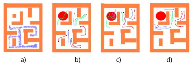
Visualization

a) Offlinedata   b) RandomCollection  c) GreedyCollection   d) OURS

Experimental Details

• For maze type environments considered Cost function is L1 , where for open environments like locomotion considered is L2 distance.
• For offline phase for maze type environments used offline Algorithm is TD3+BC, while for others is IQL.

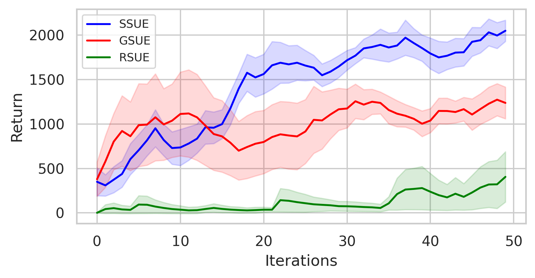
Results

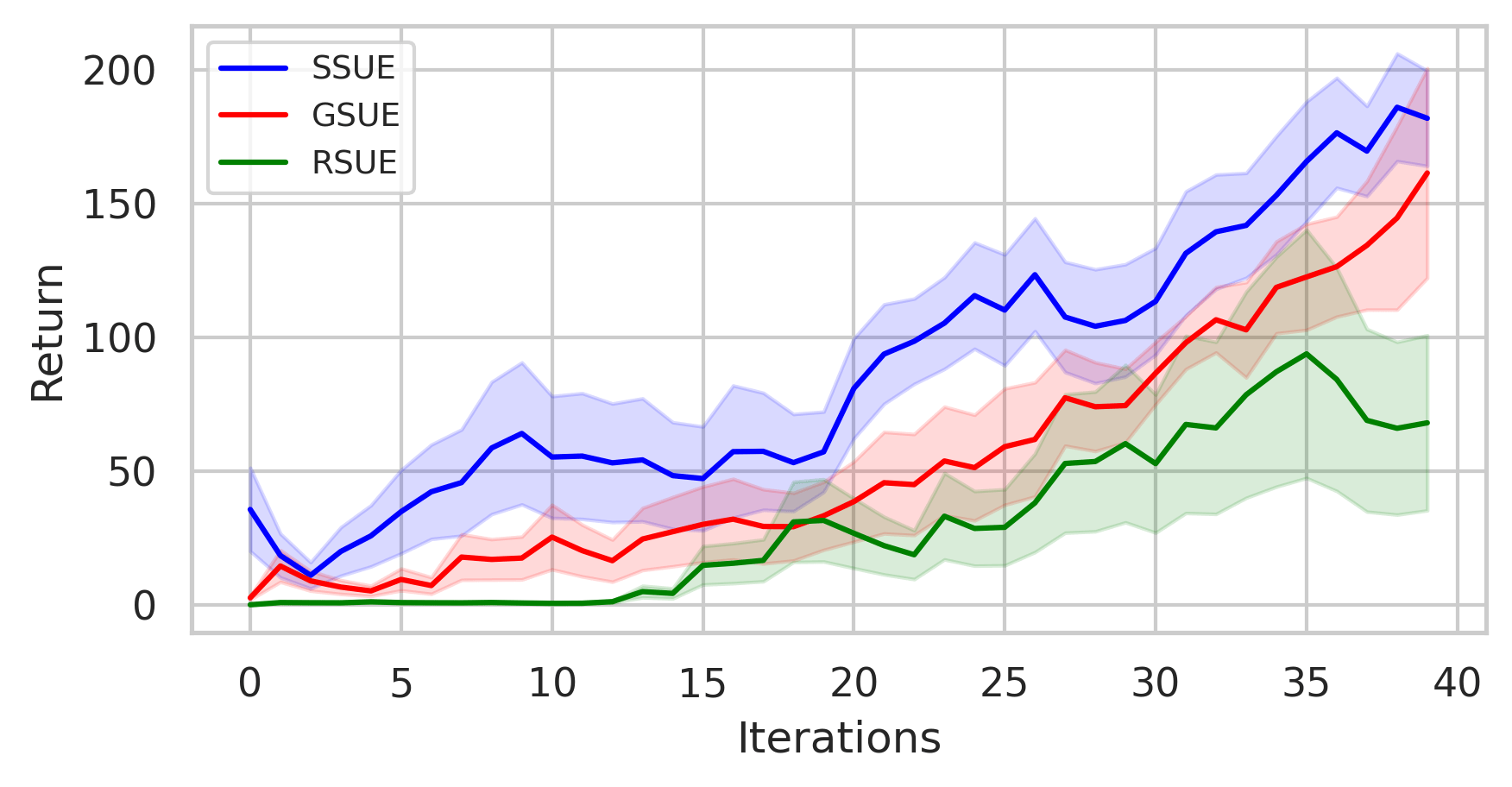
maze2d-medium                                    maze2d-hard

antmaze-play                                            hopper -medium

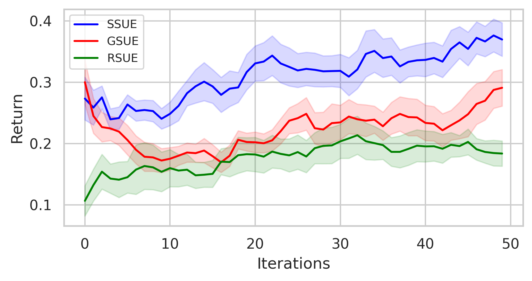
• In some environments, sample collection cost is non-uniform.
• We define a few sensitive regions centered at \( c_1, c_2, \dots, c_K \), each with radius \( r_i \). For any candidate state \( s_i \) falling inside such a region, the cost is increased as follows:

\[E'_{\text{Cost}}(s, s_i) = E_{\text{Cost}}(s, s_i) + \frac{\alpha}{E_{\text{Cost}}(s_i, c_k) + \varepsilon}\]

Non-Uniform Cost Settings

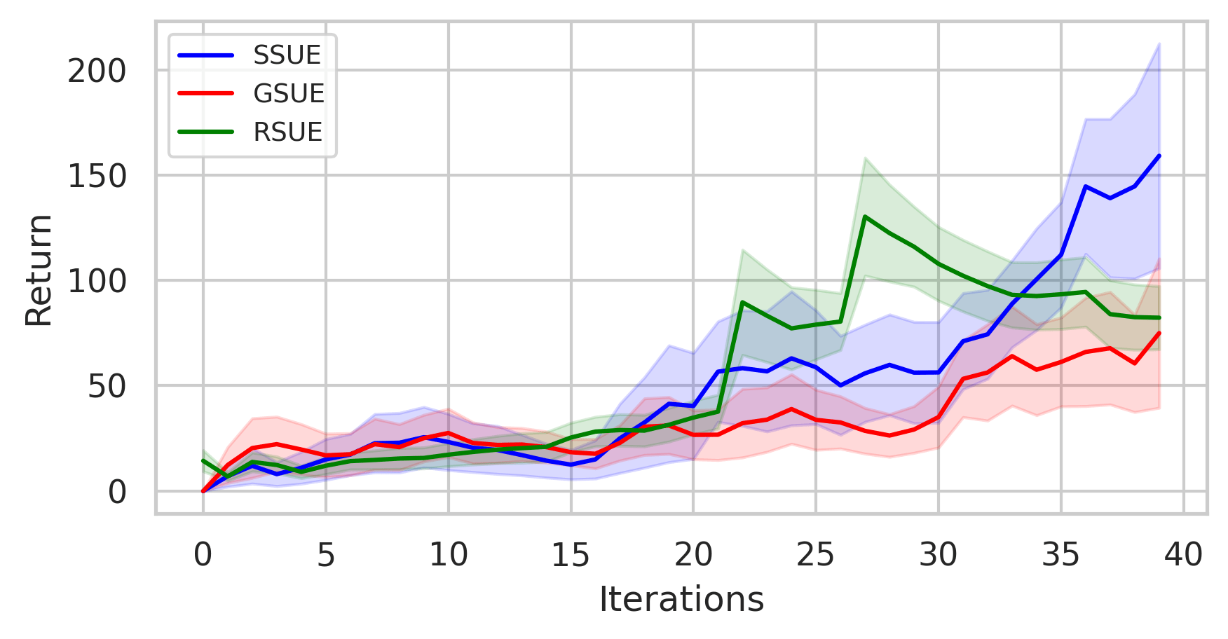
Results

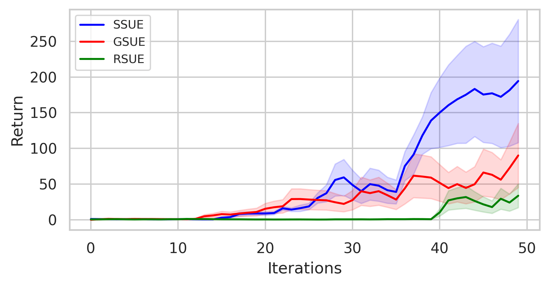
antmaze-medium                                    maze2d-hard

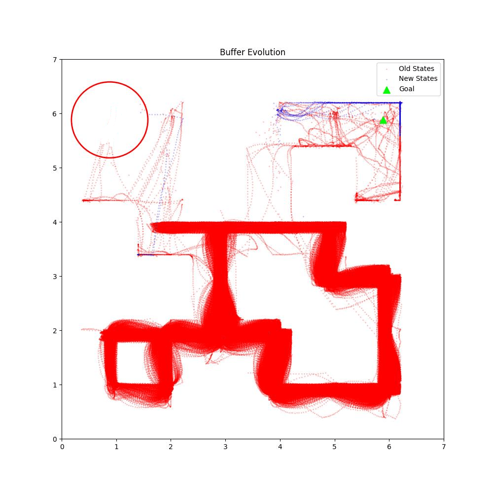
Buffer Evolution Comparsion

BaseLine                                           OURS

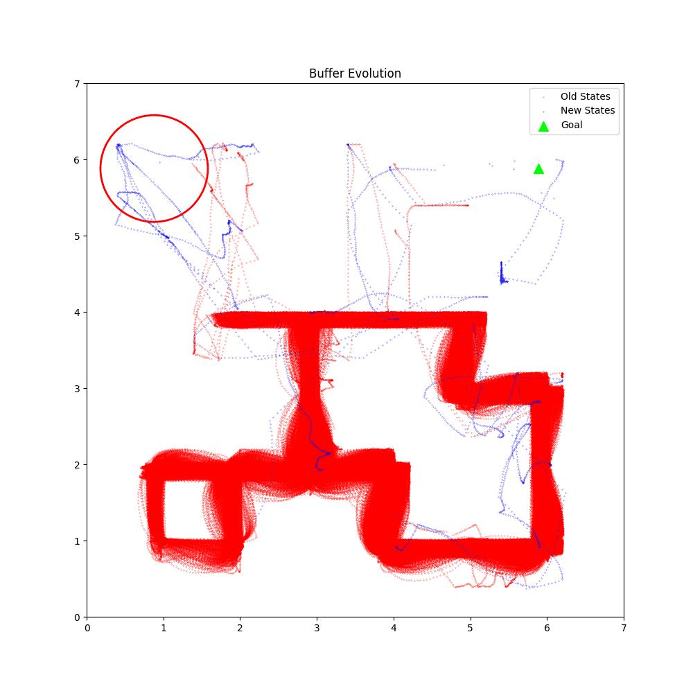
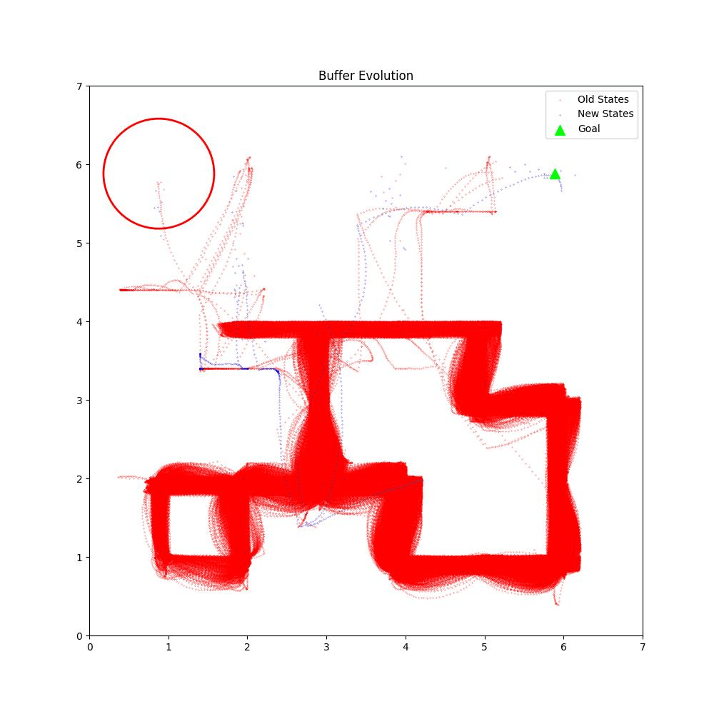
Buffer Evolution Comparsion

BaseLine                                           OURS

Conclusion

• We introduced a novel data acquisition framework for offline RL  where the objective is to collect informative trajectories while effectively utilizing the budget provided to the agent in the environment.

• Unlike traditional methods, our approach jointly solves selection and planning, enabling efficient trajectory collection in optimal sequence.

• Empirical results show consistent policy improvement across environments, demonstrating effectiveness even under non-uniform cost settings.

THANK YOU